
Sparse Attention: Algorithm–Infra Co-design
Aug 10, 2026
TL;DR
- More sparsity does not necessarily mean more speed. Reducing computation is only half the problem. End-to-end performance also depends on whether the selected data can be moved and reused regularly, and on how much work it takes to find that data.
- NSA creates regularity before loading the data. It selects contiguous 64-token blocks and shares each selection across 16 query heads, allowing the sparse workload to map directly to a regular GPU tile.
- DSA reconstructs regularity after loading the data. It permits arbitrary token selection but shares token IDs across all 128 main heads. FlashMLA then moves scattered rows into SMEM and repacks them into regular tiles. The cost is that Discovery (Indexer plus exact Top-K) must still scan every candidate.
- DSA’s bottleneck is not strongly tied to address randomness; it lies in finding the selected tokens. In the tested H100 sparse-prefill configuration, latency point estimates for eight random row permutations stayed within 0.47% of sorted access. In the public DSA pipeline, however, Discovery (Indexer plus Top-K) was already slower than FlashMLA at the 64K checkpoint, and the gap widened rapidly with context length.
- The system must therefore optimize Discovery, not only the final sparse kernel. At the systems level, fusing the Indexer with Top-K can avoid writing and rereading the complete FP32 score matrix. At the algorithmic level, each query must avoid scanning the entire KV history. The former reduces constant-factor overhead in the current implementation; the latter can fundamentally change long-context scaling.
1. Opening
Sparse Attention is easy to write down. The hard part begins when the selected KV entries no longer form a regular matrix: how should a GPU load them, compute with them, and reduce their gradients? NSA and DSA answer that question through two different co-design paths.
- NSA creates regularity before the load. Contiguous 64-token blocks and 16-head shared selection let the algorithm map directly to a regular tile.
- DSA reconstructs regularity after the load. All 128 main heads share the selected token IDs, and FlashMLA moves scattered rows into SMEM before computing on them. The cost is that candidate discovery—Indexer plus Top-K—can still grow quadratically.
Together they lead to the central claim of this article:
A sparsity ratio tells us only how much computation was removed. Actual speed depends on whether the selected data can be moved and reused regularly—and on how much work it takes to discover that data in the first place.
We first establish a common way to read tensors and tiles, then derive the algorithmic dataflow, kernel ownership, and memory movement of NSA and DSA. Two H100 experiments appear only where they answer a specific question: one tests how sensitive the DSA sparse kernel is to selected-row address patterns; the other tests how the quadratic Discovery term hidden behind the sparse main kernel grows with context length.
This article does not re-explain dense Attention or FlashAttention. It begins where
block IDs and token IDs are produced and asks how a kernel consumes them. [PAPER],
[CODE], [DERIVATION], and [MEASURED] mark claims from papers, public code,
our derivations, and formal measurements.
2. Three Concepts Are Enough to Read the Rest
Many shapes appear below, but the reading method has only three parts.
A program is one independent Triton kernel instance; in CUDA terminology it is roughly one CTA (thread block). SMEM is on-chip memory shared within a CTA. HBM/global memory is larger and slower device memory.
First, a logical tensor is not necessarily an HBM tensor. One Attention row has
and logically produces and . This does not mean that or must be written to HBM. We will distinguish the logical shape defined by the algorithm, the materialized shape preserved across kernels, and the tile shape processed by one CTA/program.
Second, every output needs an explicit owner. Here the owner is the program that ultimately writes that output region. Suppose one program owns softmax rows and streams over KV entries at a time:
With score scale , the local work is always two regular matrix products:
The program keeps only the online-softmax state for the rows it owns:
As each KV tile arrives, it updates the row-wise maximum , rescales the old and to the new maximum, and accumulates the current probabilities and value numerator. Selected blocks or rows can therefore stream in without materializing the complete probability matrix.
Third, the key question is not only “how much was skipped?” but “where does irregularity stop?” For each path we track four things:
- how selection is produced and whether it materializes an intermediate tensor;
- what output one program owns;
- how many rows or heads reuse one KV load;
- where a dynamic index becomes a regular tile again.
We count one FMA as 2 FLOPs. Unless noted otherwise, byte counts use BF16 useful payload; cache-line overfetch, page/TLB behavior, and allocator effects are discussed where they matter.
3. NSA: Make the Algorithm Produce an Executable Block Workload
Takeaway. NSA is not efficient merely because it “selects 16 blocks.” Each ID names 64 contiguous tokens, and all 16 heads in one KV group share those IDs. The algorithm therefore already produces something close to a regular interaction tile.
NSA decomposes long-context Attention into three access patterns:
The key derivation is not merely “sum three branches,” but
The algorithm comes from the NSA paper. The kernels used in the paper’s experiments
are not fully public, so our code-level discussion of online Top-K, the forward grid,
and backward uses the FLA community implementation as one concrete path. Choices
specific to that implementation are identified explicitly.
[PAPER] [CODE/community] [GAP]
3.1 Algorithmic Contract: What Each Sparse Branch Contributes
Omitting the batch axis and using a sequence-major layout, a sequence of length has
NSA targets GQA. The paper’s efficiency experiments use
The query-head group corresponding to KV head is
The algorithmic parameters of the three branches are:
| Branch | Sparse unit | Paper configuration | Visible extent per query |
|---|---|---|---|
| compression | overlapping window | approximately | |
| selection | contiguous token block | at most | |
| sliding | local token window | at most 512 |
Here is the length of the causal prefix at position . It contains
complete compression windows, and
causally visible selection blocks.
The three branches are not three masks over one shared KV representation. The paper gives each branch its own K/V projection:
Therefore, even if multiple branches access the same token, we cannot first take a union of token IDs and treat the result as one attention operation. The branches use different representations, normalize independently, and only then combine their outputs.
Compression answers “what is roughly present far away?” Each KV head maps an overlapping window of length through a learned compressor into one compressed K/V row. Adjacent windows have stride , so a full sequence produces approximately compressed K/V rows.
The local shapes for position and group are
With a fixed stride , the total compression workload across all queries remains
It is smaller than dense attention by a constant factor of roughly , but it is not linear in sequence length.
The sliding window answers “what is happening nearby?” The local branch accesses only
providing fixed, contiguous local context that tiled attention can handle naturally.
Selection answers “which distant details should be expanded again?” Each branch performs its own softmax and produces
which are then combined by independent sigmoid gates:
These gates need not sum to 1. In the execution DAG, compression attention and sliding attention can run in parallel; selection attention must wait for the routing IDs.
3.2 Routing: From Compression Probabilities to Top-16 Block IDs
Selection does not train another router. It reuses compression-Attention probabilities to convert “which compressed windows matter?” into “which 64-token blocks should be expanded?” The process has three steps: spatial remapping, a 16-head reduction, and Top-16.
Spatial remapping. Let
be the compression probability for query head . Equation 9 of the paper converts it into a selection-block score:
An out-of-range compressed-window index is treated as zero. The paper’s configuration satisfies
This double sum handles the fact that overlapping compression windows and selection blocks do not correspond one-to-one.
GQA group reduction and Top-. The query heads sharing a KV head must use the same selection IDs, so
The concrete configuration in Section 4 of the paper further specifies that, among the 16 selection slots, one initial block and the two most recent local blocks are always active; only the remaining slots are filled by the dynamic ranking above.
[PAPER]
The fixed initial block deterministically creates a hot row with fan-in. The two local slots move forward with the query: under the current-plus-previous rule alone, any particular block serves at most about query positions. Dynamic ranking can create additional hot spots.
[DERIVATION]
At a mature position,
This is an index tensor with an explicit slot order, not a mathematical set. Near the beginning of a sequence, fewer than 16 causally valid blocks may exist. The kernel may still maintain 16 selection slots, but padding must be marked by or by a block count. “A fixed 16 slots” does not mean “16 valid blocks always exist.”
The complete shape chain is
compression probabilities       [T,Hq,≈T/16]
  → Eq. 9 spatial remap          [T,Hq,≈T/64]
  → reduce G=16 query heads      [T,Hkv,≈T/64]
  → Top-16                       [T,Hkv,16]
But where are the probabilities? Standard FlashAttention does not write the complete probability matrix back to HBM; it usually returns only the output and LSE. Therefore, “reuse the compression probability” does not by itself explain how that probability reaches Top-k.
At , the actual number of complete windows is . To illustrate the upper bound for a fixed-shape allocation, let the padded capacity be
Materializing per-head FP32 compressed scores at that capacity,
requires
per layer.
If we first sum over each GQA group before the Equation 9 remap, materializing
still requires
If instead we are discussing group-reduced block scores after the remap, let . Their shape should be
corresponding to
These three numbers describe different locations in the dataflow and must not be conflated.
The current FLA implementation demonstrates one feasible mechanism: save the compression LSE, recompute probabilities in blocks from Q and compressed K, and maintain Top- online using bitonic merges, thereby avoiding materialization of the quadratic score tensors above. This path trades recomputation for memory capacity: the Top-k kernel must scan compressed K with Q once more, so routing still contains a QK scan and candidate merging. It eliminates HBM materialization of the quadratic score tensor, not quadratic pair scoring itself.
The accompanying path also simplifies compression to non-overlapping mean pooling, shares K/V, and imposes implementation constraints that the GQA group size be at least 16 and a power of two. None of these is part of the paper algorithm’s general definition. FLA therefore proves only that one infrastructure path is feasible; it does not prove that the paper authors used the same implementation. [CODE/community] [GAP]
3.3 Selection Forward: Logical Gather, Physical Block Tile
From 16 IDs to 1,024 Logical Tokens
Routing produces discrete block IDs:
Each points to a contiguous 64-token block in selection K/V:
For a mature query with all 16 slots valid, the logical gather is
The logical attention shapes are
Here 1024 is the padded capacity, not the number of valid tokens at every position. Some slots may be invalid near the beginning of the sequence, and a causal block containing the current position may expose only part of its tokens. An implementation must apply the ID mask, range mask, and causal mask together.
The above is only the logical shape after concatenation. In the original KV storage, it corresponds to 16 mutually disjoint 64-token blocks, each internally contiguous in token index; it is not one contiguous 1,024-token source range. If the physical layout is token-major , adjacent token rows for a fixed head have a fixed stride and need not form a byte-contiguous interval. What the algorithm truly improves is the addressing structure: one block requires only one irregular base address, from which 64 rows are expanded by regular affine offsets, rather than 64 separate indirect token lookups.
If we actually constructed these two tensors for every query/group, the external gather would need both to handle 16 irregular block bases and to assemble them into a compact selected-KV tensor written back to HBM. The K/V payload alone would be
in BF16. This creates an extra write, after which attention reads the same data again. The correct approach is to retain only the IDs and load the original K/V by block inside the attention kernel.
What Does One Program Ultimately Write?
The most natural owner for selection forward is
We first expand all input shapes and grid symbols used by this source path. For fixed-length inputs, FLA uses
Here:
- is the batch size;
- are the numbers of query and KV tokens per sequence in the current invocation;
- are the numbers of query and KV heads;
- is the number of query heads served by one KV head;
- are the Q/K feature and V/output feature dimensions per head;
- is the slot capacity along the final dimension of the selection-ID tensor, written as
Sin the source; the configuration here uses 16; - stores block IDs. When
block_countsis a tensor, it records the number of valid slots for each query/group. When it is a scalar capacity, the kernel scans all slots; - is the tile width that one program computes along the value-feature axis;
- is the number of tiles required to cover the complete value dimension.
The NSA numerical configuration used here is
FLA further assumes that corresponds to the last tokens of each KV sequence. Thus, on the fixed-length path, the absolute position of query slot within the KV sequence is not simply , but
The subsequent causal mask and selected-block start positions are both evaluated relative to .
The launch grid in the source is a three-dimensional program-count tuple:
The source names the three program IDs i_t, i_v, and i_bh. To avoid confusing
i_v with the value tensor , we rename the second ID :
They represent, in order, the query position, the value-feature tile, and a flattened batch/KV-head position. The third ID is unflattened as
to recover batch index and KV-head/group index . We intentionally use for the batch here to avoid confusion with the KV block ID below. The query heads served by group remain
Next define the value-feature interval owned by program :
Program , equivalently , is then the unique writer of the following output slice:
The physical accumulator is allocated as ; a final tile narrower than is handled by a feature mask. This also makes the axis order explicit: after removing batch flattening, the grid is , not .
If , the same expands into programs. Each program recomputes the same QK/softmax for its own value-feature slice, but the intervals are disjoint, so there is no output write conflict. LSE is not tiled along the value dimension; the source permits only the program to write .
The paper uses , and the current FLA path also takes , so
Each then corresponds to exactly one program, which exclusively owns the complete selection output . The program subsequently loads and keeps resident the logical query tile
Optional implementation note: variable length does not change ownership. The public variable-length path uses a packed representation. If sequence contains query tokens and KV tokens, respectively, then
The grid then becomes
The first program ID is a packed query slot;
token_indices_q[u] maps it to
. Let
denote the starting offset of sequence in packed Q. The physical output owner is then
The corresponding causal absolute position of this query within its sequence’s KV storage is
Thus, varlen changes only how fixed-length coordinates are located. The and grid axes, and the ownership rule that “one program uniquely writes one output slice,” remain unchanged.
How a 64-Token Block Becomes a Regular Tile
The program then loops over the 16 selection slots. We use for the number of KV-token rows loaded and computed in one inner-loop iteration. In the current FLA path, it corresponds to the source parameter BS and exactly equals NSA’s selection block length :
For a valid block ID , the program computes and loads
This is the logical tile at the algorithmic level. In the current Hopper branch of FLA,
so matching Triton’s dot-product feature tile requires the physical construction
where the tail of the feature dimension is handled by masking/padding. The logical contractions are therefore
The physical padded execution shape for QK is
This execution shape is a conclusion about the current FLA Hopper path. The non-Hopper branch caps BK at 128; with , it produces two feature tiles and triggers the source’s NK == 1 assertion. The
shape therefore cannot be extrapolated directly to that path.
The only dynamic component is the block base computed before each load. Once the data reaches the on-chip tile, computation returns to a fixed shape.
We deliberately do not use for the token tile here. The NSA paper’s token-tile notation corresponds to BS in the current FLA source, whereas FLA’s BK denotes the padded feature width—for example,
Mixing the two notation systems would mistake “64 tokens” for “256 feature elements.”
Online normalization. Across the 16 blocks, the program uses the exact online-softmax merge introduced above. It maintains only the running maximum, normalizer, and output accumulator for each query head; it does not write . After all selected blocks have been processed, it directly writes
The output therefore has a unique writer, and the forward pass needs no atomic reduction on the output.
Why head sharing is an execution contract. For one 64-token block, the QK and PV multiply-add count is approximately
With BF16 K/V, the primary K/V payload for this iteration is
Considering only the K/V payload shared by 16 heads, the local arithmetic intensity is
This is not a roofline figure for the entire kernel: it excludes Q, output, indices, LSE, masks, and launch overhead. It only shows that the more query heads reuse the same K/V block, the more easily the cost of one irregular address lookup is amortized by regular matrix multiplication.
For a mature query, the main selection loop has 16 slots. Near the beginning of a sequence, the same control structure still runs, but invalid slots are masked. NSA provides a “fixed-capacity, padding-compatible workload,” not an absolutely fixed amount of work without boundary conditions.
3.4 Forward and Backward Use Different Sparse Graphs
Takeaway. The forward relation
query → selected blocksfinds an owner only for the output. If we retain query-centric ownership, requires floating-point atomics or a partial-gradient reduction. The FLA community implementation audited here instead transposes the relation intoKV block → selecting queries, then lets each KV-block program perform its own many-to-one reduction.
The natural owner in the forward pass is the query, because each program can independently complete one . The backward pass, however, has two reduction directions.
The discussion below covers only the backward pass of the selection branch. Complete NSA also includes gates, a compression branch, a sliding branch, and the merging of gradients from all three branches into shared Q/input tensors.
Recompute Probabilities, Preserve the Sparse Graph
Selection backward does not need to save the complete probability matrix. It recomputes score/probability tiles from , and , then combines them with to recover local gradients. For batch/sequence , query , group , and selected block , the local shapes are
Without activation checkpointing, the FLA selection autograd state includes at least
as well as block counts and sequence metadata required in variable-length cases. The current FLA autograd path actually saves q, k, v, o, lse and retains metadata such as block indices in the context. The accurate conclusion is “ is not saved,” not “the forward pass only needs to save
.”
: the Query Remains the Owner
For query , only the blocks it selected contribute:
The local shape for each block is
The same program can loop over all slots and accumulate
in registers before writing it back exactly once. Thus, dQ remains well suited to query-centric ownership.
Why Cannot Remain Query-Owned
One KV block may be selected by many queries. Define
Its gradients are many-to-one reductions across queries:
Transpose the Sparse Graph and Make Each KV Block the Owner
If we keep the query as owner, different programs update the same concurrently. The implementation must then use many floating-point atomics or write partial buffers and reduce them later. A more natural approach is to transpose the sparse relation first:
forward adjacency:   query → selected KV blocks
backward adjacency:  KV block → all selecting queries
and then assign one program to each KV block.
CSR representation. Let the batch size be , and let the number of blocks in a complete sequence be
The padded shape of the input IDs is . The upper bound on edge capacity allocated for csr_indices by the current FLA implementation is
The actual number of valid edges is determined by the ID range, block count, and causal condition:
Flatten into a one-dimensional row:
The CSR metadata shapes are
where only is a valid prefix. Row corresponds to
This is one-dimensional flattened CSR. It must not be written as a nonexistent two-dimensional index .
CSR is constructed with two counting/scatter passes:
traverse valid selection edges
  → atomically count the fan-in of each (batch,group,block)
  → prefix sum to obtain csr_offsets
  → traverse the edges again and scatter query IDs using an atomic cursor
Atomics operate only on compact integer metadata; the expensive floating-point reductions for obtain a unique owner.
Take
Then
so the int32 csr_indices buffer allocated by the current FLA implementation is 16 MiB.
For a complete causal self-attention sequence, suppose early positions use all distinct visible blocks. The first 15 query blocks of 64 tokens then have valid slots respectively, after which the count reaches 16. In this case,
This number is smaller than the allocation upper bound; the two should not both be denoted by the same .
Meanwhile,
int32 offsets require only about 16 KiB. For comparison, materializing a uint8 inverse mask of shape requires
CSR reduces inverse metadata from to , at the cost of two edge traversals, integer atomics, a prefix sum, and subsequent irregular query gathers.
KV-centric dKV tile. A dKV program owns
and gradient accumulators of the same shapes. It reads query positions at a time from the corresponding CSR row and expands the heads of each query:
The batched query and output-gradient shapes are
Local recomputation and reduction once again form regular matrix multiplications:
For example, when , we have , and the central score-recomputation tile is
CSR does more than compress metadata. It rewrites the conflict “many queries write the same KV-gradient address” into “one KV owner sequentially reads its own queries,” and then restores a regular Tensor Core tile within that owner.
Write Conflicts Disappear; the Fan-in Tail Remains
Define
When block_counts=16 is a fixed scalar capacity, each
program scans 16 padded slots. FLA also accepts a per-query tensor block_counts, in which case the runtime may be shorter. The loop length of a dKV program, by contrast, is determined by . A fixed initial/sink block, as well as popular blocks created by dynamic ranking, may have fan-in far above the mean and form long-tail CTAs; the moving local slots themselves create only bounded local fan-in. Splitting a hot row can improve load balance but reintroduces a partial reduction or atomic operations. The backward problem therefore changes from “how many FLOPs can be skipped?” to “how should a many-to-one reduction be scheduled?”
We do not turn this long tail in fan-in into a performance experiment here. On the one hand, the backward kernel used by the paper’s authors is not public. On the other hand, changing the routing topology in the community implementation changes fan-in skew, query-gather locality, and CSR row order together, making it difficult to attribute latency differences to a single variable. FLA backward therefore moves irregularity from floating-point write conflicts into CSR row length, query-gather locality, and CTA load balance. We report no performance measurement for these factors; we treat them only as execution consequences confirmed by the source and do not claim that they explain the backward latency of the paper authors’ kernel. [DERIVATION] [CODE/community] [GAP]
3.5 NSA’s Regularity Comes from the Algorithmic Contract, Not Kernel Magic
Under the paper’s default configuration, NSA selection maps efficiently to a kernel because the algorithm deliberately provides three execution contracts:
The forward pass brings dynamic block bases into the program’s inner loop and restores regular computation after the load. The FLA community backward path analyzed here then transposes the sparse graph so that a KV block becomes the unique owner of .
This also reveals three boundaries that must not be crossed.
First, NSA is not evidence that “arbitrary block sparsity automatically accelerates.” Hardware efficiency arises only when contiguous blocks, head sharing, a fixed slot capacity, and explicit ownership all hold simultaneously.
Second, the token budgets of the selection and sliding branches are approximately fixed at mature positions, but compression still accesses roughly compressed K/V rows. For fixed , full-layer compression remains .
Third, FLA demonstrates a complete feasible mechanism comprising online Top-k, group-centric forward, and CSR backward. It cannot prove that the paper authors’ unreleased implementation uses the same routing materialization, tile parameters, or inverse-adjacency construction.
The paper reports that, with its configuration and on its A100 test environment, the authors’ Triton NSA reaches 9.0× forward and 6.0× backward speedup over Triton FlashAttention-2 at 64K. This result can be attributed to the complete system reported in the paper; it cannot be attributed directly to any single kernel choice isolated from the community code in this article. [PAPER] [GAP]
In other words, the most reusable part of NSA is not one particular sparsity formula, but a co-design method:
First make the algorithm emit sparse units that a GPU can consume, then choose a unique owner separately for the forward output and the backward gradient.
4. From Blocks to Tokens: Why DSA Can Use Finer Selection
NSA and DSA are not simply an “old design” and a “new design.” NSA selects blocks so that training and inference can consume contiguous tiles directly. DSA selects tokens because MLA exposes a different and sufficiently strong reuse axis. The hardware constraint did not disappear; the algorithm changed how it satisfies that constraint.
4.1 Infra: Contiguous Blocks Are No Longer the Only Source of Regularity
Consider the problem NSA faced. Arbitrary token selection creates many scattered KV
rows, and during training those rows also participate in the backward reductions for
. NSA therefore fixes the selection unit to a contiguous 64-token block. The
cost is that selection can say only “this region matters,” not select just the
relevant tokens inside it. NSA trades selection granularity for regularity before the
load. [PAPER]
DSA starts from a different base. DeepSeek-V3.2 already uses MLA, so each token stores
one shared latent-KV entry. DSA further makes all 128 main heads of a query share one
set of token IDs. A scattered row may be difficult to load, but after loading it can
serve many heads. FlashMLA can therefore leave random addressing to the producer while
Tensor Core consumers operate on regular SMEM tiles. Contiguous blocks are no longer
the only way to obtain hardware efficiency. [PAPER] [CODE]
From the infrastructure perspective, the design changes along three axes:
| NSA | DSA | |
|---|---|---|
| Selection unit | Contiguous token block | Arbitrary individual token |
| Reuse axis that amortizes the load | 16 query heads in one KV group | 128 main heads for one query |
| Where the regular tile appears | Before the global load | After scattered rows enter SMEM |
This finer selection is not a free upgrade. NSA routes on a compressed token axis.
DSA preserves full token resolution in the Indexer and then performs exact Top-K.
It bounds the main Attention by without removing the
Discovery term. A more accurate description is: DSA trades stronger
cross-head reuse and a specialized gather kernel for token-level selection, then
moves the system bottleneck from sparse main Attention toward the Indexer and
Top-K. [DERIVATION]
4.2 Training: Attach a New Router to an Existing MLA Checkpoint
DeepSeek did not train DSA from scratch. It continued from DeepSeek-V3.1-Terminus after extending that model to a 128K context:
- Dense warm-up: keep dense Attention, freeze the main model, and train the Indexer with a KL objective derived from the dense-Attention distribution.
- Sparse training: enable Top-2048 and let the main model adapt through the language-modeling loss; the Indexer continues to use a separate KL loss. Its input is detached from the main-model graph so that the two gradient paths remain isolated.
The point of this procedure is to retain the existing MLA parameterization while
adding a router and a sparse kernel, rather than training the entire Attention system
from scratch. [PAPER]
Evidence boundary. The DeepSeek report does not provide a direct NSA-versus-DSA ablation or enumerate reasons for abandoning NSA. What is public is each paper’s algorithmic contract, DSA’s use of MLA/MQA sharing, and its continued-training procedure. The explanation above—why the design can move from blocks to tokens—is a systems inference from those facts.
We can now follow the actual DSA dataflow: Indexer scores, Top-K token IDs, the MLA execution representation, and finally the FlashMLA kernel.
5. DSA: Turn Arbitrary Token Selection Back into Regular Matrices
Takeaway. DSA permits arbitrary token selection but makes all 128 main heads share one set of IDs. Only the FlashMLA producer handles scattered addresses; once rows enter SMEM, the consumer still sees regular matrices.
The complete DSA forward path has three stages:
The table below keeps only the notation needed to follow those shapes.
| Symbol | Meaning | DeepSeek-V3.2 |
|---|---|---|
| Number of queries in the current call and number of visible KV tokens | Determined at runtime | |
| Number and dimension of Indexer heads | ||
| Number of main MLA query heads | ||
| Latent-KV and RoPE dimensions | ||
| NoPE dimension of the original main MHA | ||
| Value dimension of the original MHA | ||
| Maximum number of tokens selected per query |
must not be confused with FlashMLA’s latent-value dimension . The main Attention also has two algebraically equivalent representations with different execution shapes:
5.1 Indexer: Low-Dimensional, but Still Scanning the Full History
Step 1: Score Every Query–Token Pair
The Indexer assigns a cheap routing score to every visible token and selects Top-:
where
Across all queries and visible tokens, the final routing-score matrix is . Projection, RoPE, Hadamard, FP8, and DeepGEMM fusion all serve the same goal: compute this matrix without writing the much larger intermediate to HBM.
One DSA layer also contains two distinct kinds of scores:
and
is the Lightning Indexer’s routing score, used only to produce token addresses. is the attention logit recomputed by the main MLA over the selected tokens, and only this score enters the main Attention softmax.
The Indexer therefore decides where to look, not how to weight what is found.
Step 2: Produce Low-Dimensional Queries, a Shared Key, and Head Weights
The normalized hidden states
first produce the low-rank query latent shared by the main MLA and the Indexer:
Rather than performing another large projection directly from the 7168-D hidden state, the Indexer derives its query from :
After reshaping:
The released DeepGEMM interface takes a materialized FP8 Q as input. The public code does not reveal whether the production system further fuses this projection, rotation, and quantization.
Each historical token, by contrast, has only one shared Indexer key vector:
The persistent cache has logical shape
Thus, the 64 Indexer query heads share one historical key rather than maintaining a separate K cache for every head.
The Indexer also projects query-dependent head weights directly from the current hidden state:
is the base weight of Indexer head for query ; this branch does not pass through a softmax. Absorbing the two fixed normalization factors used by the official reference, define
Only Indexer Q reuses . Indexer K and these weights are both projected directly from .
Step 3: RoPE, Hadamard, and FP8
Each 128-D Indexer Q/K vector is split as
The first 64 dimensions use non-interleaved RoPE, unlike the interleaved RoPE used by the main MLA. This is not a notational detail: if the two sides use different pair layouts, their dot product at a given position changes.
After rotation, a normalized Hadamard transform is applied:
Before quantization, therefore,
The Hadamard transform does not change the exact real-valued inner product; it spreads outliers so that subsequent E4M3 quantization is more stable. “Inner-product preserving” must not be extrapolated to mean “bitwise identical after quantization.”
A note on the two symbols named . is a scalar—the number of Indexer heads. is the Hadamard transform matrix. Its entries are ; it is fixed, orthogonal, and not learned. The implementation need not materialize this matrix. A fast Hadamard transform evaluates it through hierarchical additions and subtractions in time. Q and K use the same after partial RoPE and before FP8 quantization, so the real-valued inner product is preserved exactly before quantization and only approximately afterward.
Let denote the E4M3 data, and let denote the corresponding scales. The official reference folds the query scale and both normalization factors into the query-dependent weight:
The scorer’s implementation semantics can then be written as
Here, explicitly refer to vectors after partial RoPE, Hadamard transformation, and FP8 quantization; they are no longer interchangeable with the pre-transform .
The logical payload of one Indexer K-cache entry is
Compared with a full main-KV row, this is what makes the bandwidth of the full-history scan substantially smaller.
Step 4: Fuse 64 Heads On Chip and Write Only the Final Score
Mathematically, for a fixed query , we first have
The global logical shape is
After ReLU, weighting, and reduction across heads:
Writing to HBM would make the low-dimensional Indexer create an intermediate 64 times larger than its final score tensor. The released DeepGEMM scorer therefore fuses the matrix multiplication, ReLU, query-dependent weighting, and 64-head reduction, writing only the final FP32 .
One of its core tiles, expressed in the GEMM direction used by the code, can be summarized as
The final step applies ReLU, query-dependent weighting, and reduction over the 64 Indexer heads, then maps candidate-major accumulator fragments directly to the logical output addresses. There is no separate transpose stage. The intermediate 64-head result remains on chip; HBM sees only the final score tile for two queries and 256 candidates.
The released scorer, however, does not include Top-K. The public DeepGEMM pipeline still allocates and materializes the complete rectangular carrier
The main scorer writes the legal candidate range of each row. When
clean_logits is enabled, a separate cleanup kernel fills invalid and future regions.
Exact Top-K then scans the complete rectangular result again.
DeepGEMM has therefore implemented fusion within the scorer: FP8 matrix multiplication, ReLU, query-dependent weighting, and 64-head reduction occur in one kernel, and the per-head scores are never written to HBM. But this is not Indexer–TopK fusion. The released scorer still emits the full , which a separate exact Top-K implementation must scan again.
Step 5: Top-K Turns Scores into Token Addresses
For query position , let be the final causally visible position. Mathematically,
is a token address, not a routing score. All 128 main heads of the same query share , while the selected sets of different queries can be entirely different.
The public interface also requires two shape/dtype adaptations.
First, torch.topk in the official inference reference returns INT64 indices and uses
min(index_topk, end_pos) for the fixed trailing dimension of one call; the causal
mask keeps future positions invalid.
Second, under the DSA configuration studied here, FlashMLA sparse-prefill accepts a fixed width :
If a row has only legal tokens, all remaining slots must be replaced
by an invalid sentinel, such as -1 or
an address no smaller than . Repeating a legal token to fill the row is
incorrect, because the softmax would count that token more than once.
Converting the reference’s INT64 Top-K result into a fixed-width INT32 kernel tensor is therefore real data-preparation work, not a dtype annotation that can be omitted from a shape diagram.
Top-K IDs are discrete control flow. Except at sorting boundaries, the language-modeling loss cannot provide an ordinary continuous gradient through the decision of whether a token is selected. During dense warm-up, the main model is frozen and the Indexer is trained with a KL loss against a target obtained by summing dense attention over the main heads and L1-normalizing along the sequence axis. During the sparse stage, the main model trains on the language-modeling loss while the Indexer continues to train on a KL loss restricted to the current selected set. The paper explicitly detaches the Indexer input, so the Indexer receives only while the main model receives only the language-modeling loss. The main model therefore adapts to sparse selections produced dynamically by the current Indexer, not to a fixed set of token IDs. This explains how routing is learned, but it does not change the execution cost of exact Top-K at inference time.
5.2 MLA Bridge: Why the Main Kernel Is 576-D MQA
The Original MHA Form Re-expands the KV Cache
The Indexer produces addresses; the main MLA still computes the actual attention weights. FlashMLA’s input shapes become clear only after rewriting MLA from its original MHA form into an equivalent MQA execution form.
Start from the original score. The shared query latent is projected by
Each head is split into
where receives the main MLA’s interleaved RoPE. On the KV side,
RMSNorm turns the first 512 dimensions into , while RoPE turns the final 64 into . The cache therefore stores
If expanded into ordinary MHA, each head would construct
with
The resulting tensors would have shapes
Materializing them for all 128 heads would discard the cache compression before attention even begins.
Absorb the Key Up-Projection into the Query
The content score satisfies
Define
then concatenate the RoPE component:
The QK execution shapes are now
The singleton head dimension means that every main query head uses the same MQA key row.
The executed dot product is 576-D, but its scale is still defined by the original 192-D MHA score. In the released reference,
and
Using would change the model: 576 is the width of the absorbed execution representation, not the dimension that originally defined the attention score.
Move the Value Up-Projection after Attention
By linearity,
The sparse MQA core can therefore consume
and first produce
Applying each head’s recovers
After concatenating the heads, the layer output projection completes the path:
where . FlashMLA’s sparse core returns ; the recovery and projection happen outside that core.
This MQA form is an algebraic rearrangement, not a new approximation. In exact arithmetic it computes the same score and output as the MHA form, although BF16/FP8 rounding and a different operation order need not be bit-identical. The public Python reference expands K/V and uses MHA in its prefill branch; its decode branch exposes the MQA rearrangement directly. Here we use the representation consumed by FlashMLA’s sparse-prefill interface, not the literal call path of that Python prefill branch.
The rewrite exposes the central reuse relation: one selected KV row can serve all 128 main heads. Algorithmic sharing is not the same as physical sharing, however. The SM90 kernel places 64 heads in one CTA, so each loaded row is reused 64 ways in SMEM. A second CTA reads the same IDs, but the CTAs do not share SMEM; any reuse between them depends on the memory hierarchy and must not be assumed to be an L2 hit.
5.3 FlashMLA: Confine Random Rows to the SMEM Boundary
Takeaway. FlashMLA does not materialize and in HBM. The producer gathers 64 discrete rows directly into SMEM, so the consumer sees only a regular QK tile and a regular latent-PV tile.
Given , , and the shared KV representation, the mathematical program for the main Attention is short:
For one kernel call with fixed selection width , rewriting all query positions as a batched matrix program gives the complete logical shapes:
These two batched matrix multiplications contract over the 576-D QK feature axis and the selected-token axis , respectively. They define the algorithm’s semantics, but do not require either selected tensor to exist physically in HBM.
The real question is not the formula, but where should exist.
Stage 1: Inputs Are Only Q, Shared KV, and Token IDs
The audited Hopper sparse-prefill path is
flash_mla_sparse_fwd(
    q,
    kv,
    indices,
    sm_scale,
    d_v=512,
)
Its release contract is
q       : [TQ, HQ, 576]  BF16
kv      : [TK, 1,  576]  BF16
indices : [TQ, 1,  kappa] INT32
output  : [TQ, HQ, 512]   BF16
max     : [TQ, HQ]        FP32
lse     : [TQ, HQ]        FP32, log2-based
and it requires
architecture = SM90
H_KV         = 1
HQ % 64      = 0
kappa > 0
kappa % 128  = 0
D_QK         = 576
D_V          = 512
The last dimensions of Q, KV, and indices must be contiguous. An invalid index can be
-1 or any value no smaller than . These constraints are the capability
boundary of the current release kernel; they cannot be generalized to arbitrary head
counts, arbitrary dimensions, or arbitrary Top-K sizes.
Stage 2: Do Not Build Selected-KV in HBM
If a separate kernel first gathers
then a single query must write
Attention subsequently reads it again, so this intermediate tensor alone adds about
of logical global-memory traffic, before accounting for indices, Q, output, or cache misses. This 4.5 MiB estimate assumes the best external layout: gather only the fused row and treat as a view of its first 512 dimensions. A separate K tensor and V tensor would move even more data. The source-KV read is common to both designs and is not included in this comparison; cache hits may also prevent all logical bytes from reaching DRAM.
FlashMLA never creates this tensor in HBM. It moves only the 64 discrete rows needed for the current iteration into a regular
tile, which the Tensor Core consumer then treats as an ordinary two-dimensional matrix.
Stage 3: One CTA Owns 64 Heads
The SM90 sparse-prefill release uses
Its launch grid is
One CTA has fixed ownership of
The 128 main heads therefore use two CTAs, both reading the same .
The 384 threads form three 128-thread warpgroups:
| Warpgroup | Role |
|---|---|
| WG0 | Consumer: even 64-token chunk; owns output |
| WG1 | Consumer: odd 64-token chunk; owns output |
| WG2 | Producer: reads indices and moves indirect KV rows into SMEM |
When ,
selected-token chunks are organized into 16 even/odd paired iterations.
Stage 4: The Producer Gathers; the Consumer Sees Only a Regular Tile
The row base is random, but the 576 elements within a row are not. One BF16 KV row occupies
determines the base address of the next row. Adjacent selected rows may reside in entirely different cache lines, pages, or HBM partitions. Once that base address is known, however, the row’s 1152 bytes are contiguous.
The producer is therefore not performing 576 unrelated random scalar loads. In the
SM90 source, the logical 1152-B row is actually moved as nine 64-BF16 feature slabs,
each 128 B; eight threads issue 16-B cp.async copies for each slab. It is not one
1152-B bulk transaction. Conceptually, the producer performs
randomly determine the row base
→ cooperatively move a contiguous row with multiple threads
→ write it into swizzled SMEM
→ let the consumer read a regular [64,576] tile
The irregularity is confined to the global-memory-hierarchy-to-SMEM boundary; the internal shapes of QK and PV become regular matrices again.
Stage 5: Two Consumers Partition the Token and Value Axes
WG0 and WG1 both compute the full QK feature contraction:
They differ along the token axis for QK: WG0 processes the even chunk, while WG1 processes the odd chunk.
PV ownership is instead split along the value-feature axis:
| WG | Local probability | Resident FP32 accumulator | Contributions from local/remote |
|---|---|---|---|
| WG0 | |||
| WG1 |
Each warpgroup publishes one probability tile to the other. One even/odd pair therefore exchanges two tiles,
rather than moving their approximately 64 KiB FP32 output accumulators.
Online softmax still maintains . WG0 first publishes the max
from the even chunk, and WG1 merges the odd chunk to establish a pair-global max
baseline. The two warpgroups rescale against this common max, but each continues to
accumulate its own normalizer until the epilogue combines them in reduce_L(); the
two output halves are reduced there as well. The pipeline changes ownership, not the
mathematical softmax over selected tokens.
Stage 6: Pipeline the Next Gather under the Current Computation
This is not a simple ping-pong between two complete
tiles. plan.k[0] and plan.k[1] hold the even and odd 64-token chunks
of the current pair, respectively. Each chunk is further divided along the feature
axis into and , with a separate ready/free barrier for each
half. The producer moves one pair of chunks in this order:
even[0:256]
→ odd[256:576]
→ even[256:576]
→ odd[0:256]
→ next pair
As soon as a consumer finishes using one half, it publishes the corresponding free barrier, allowing the producer to overwrite that half in place with data from the next pair. In steady state, this still creates the overlap
compute pair i
        ||
gather pair i+1
but the pipeline operates at the granularity of four feature half-buffers rather than by exchanging the roles of two complete tiles. It reduces the visible latency of waiting for the next set of discrete rows to reach the Tensor Cores; it neither reduces the number of KV bytes that must be read nor changes the randomness of the selected row addresses. If L2/TLB/HBM latency exceeds the window that the computation of the current pair can cover, the consumer still stalls.
Why This Pipeline Has a Chance to Work
Within one CTA, every 576-D KV row is reused by 64 query heads. Counting only the QK and latent-PV work performed with that row, the local arithmetic is approximately
Dividing by the 1152 B useful row payload gives
This explains why “arbitrary token selection” does not necessarily force the consumer into low-intensity random memory access. The algorithm makes 64 heads share the address, and the kernel turns the same row into an on-chip tile with high reuse.
But 121 FLOP/B is only CTA-local intensity, not an end-to-end roofline number. It does not include
- the Indexer and Top-K;
- reads of the index tensor;
- Q, output, and softmax state;
- L2/TLB misses;
- cache-line granularity and the 256-B L2 prefetch hint;
- cache reuse between the two CTAs, which is not guaranteed;
- launch, scheduling, and fixed service overheads.
5.4 Controlled Experiment: What Cost Remains for Random KV Rows?
The decomposition above suggests a testable prediction. FlashMLA does not remove random row addresses, but their effect on end-to-end kernel latency may be small after 64-head reuse, SMEM repacking, and producer–consumer overlap. The experiment below measures that response; it does not isolate which mechanism causes it.
We ran the unmodified official SM90 sparse-prefill kernel at FlashMLA commit
3969f20 on one NVIDIA H100 PCIe, using
Each query receives a private, non-overlapping 128K-row KV arena. This removes cross-query overlap in selected row IDs, so one condition cannot accidentally gain more cross-query same-row cache reuse than another. It does not remove possible L2 reuse between the two 64-head CTAs serving the same query, because those CTAs request the same selected rows.
Each condition contains 10 interleaved measurement blocks with 20 matched rounds per
block, giving 200 per-call CUDA-event timings. Sixteen distinct conditions produce
3,200 observations under the same eight-slot rotating schedule. All 34 official
sparse-prefill tests, a 16-condition correctness gate, and the validation checks
passed. [MEASURED]
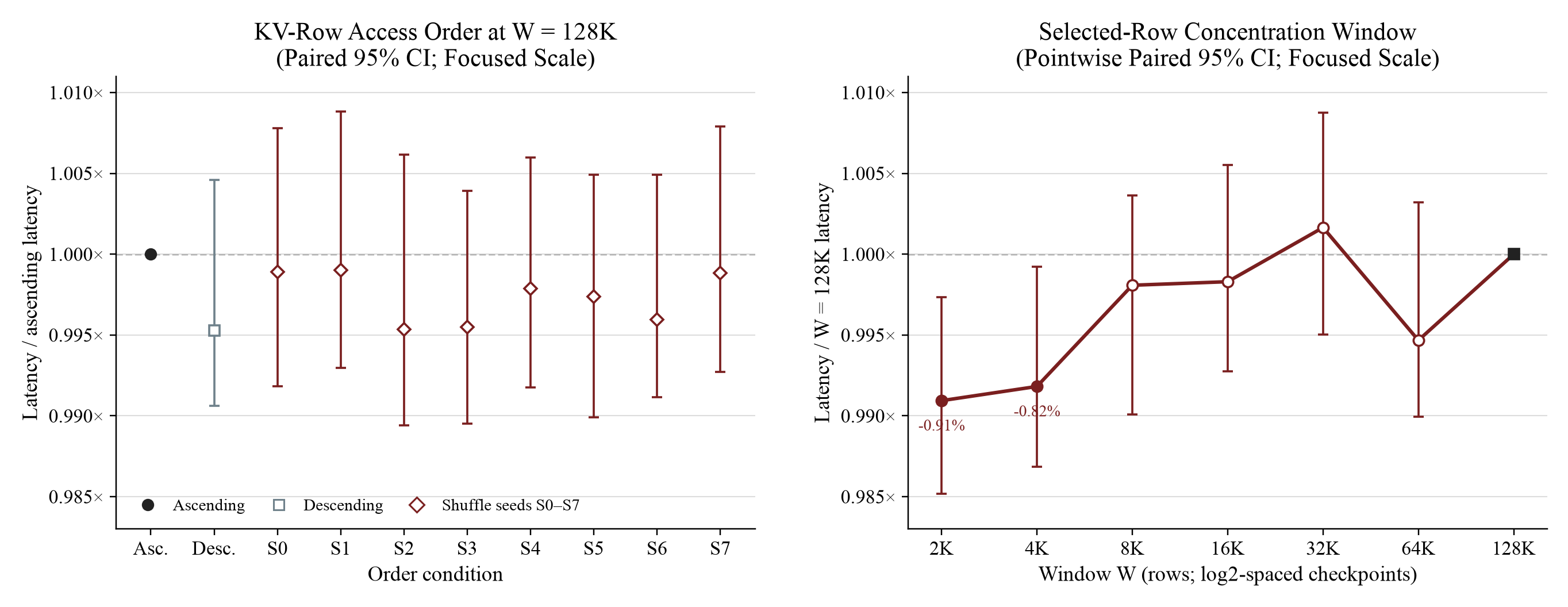
Figure 1: The focused vertical scale makes sub-percent effects visible. The left panel holds the selected-row set fixed and changes only its ascending, descending, or eight shuffled orders. The right panel changes the sampling window ; each resamples both the window origin and the exact IDs, so the line is only a visual guide, not a trajectory of one fixed selected set. Error bars are pointwise 95% intervals from a paired measurement-block bootstrap with 5,000 resamples. They are neither a population interval over all permutations nor a family-wise corrected interval.
First, change only the order. For every query and rotating slot, the left panel holds the same 2,048-row set fixed and arranges it in ascending address order, descending order, or eight independently seeded random permutations.
Ascending order has a median latency of ; descending order has . Their normalized ratio is , with a paired 95% interval of . The point estimates differ by , but the interval includes 1.
Across the eight shuffle seeds, ratios range from to , with a seed-level median of and IQR of . Every shuffle’s pointwise timing interval crosses 1. At this fixed kernel configuration, we therefore detect no latency penalty for those eight random orders relative to sorted addresses. The intervals quantify timing uncertainty for each fixed permutation. They do not describe the population of all possible permutations: only the eight seeds are independent units for permutation-to-permutation variation, while the 200 timings per seed are repeated measurements.
The near-null response is not caused by the shuffled indices remaining locally
similar. With sorted addresses, the median adjacent-row distance is 44 and a
64-index tile touches a median of 41 distinct 64-row regions. Under
W=128K, shuffle-00, these become 38,435 and 63, while the fraction of adjacent
accesses in the same region falls from to . Software-visible
locality changes by orders of magnitude; latency barely changes.
Next, change the concentration of the selected set. The right panel fixes
, uniform sampling without replacement, and the shuffle-00 rank
permutation rule, then samples rows from 64-row-aligned windows
This changes the selection distribution: each resamples both the window origin
and the exact selected IDs. It is therefore not a paired ablation in which one token
set merely changes span. Only W=128K, shuffle-00 shares exactly the same index corpus
with the left panel and serves as the baseline.
The 128K baseline has a median latency of . Relative to it, 2K and 4K windows are faster by and , absolute differences of about and . Their pointwise 95% intervals are
The other intervals include 1. Six window-versus-128K comparisons were reported without a family-wise correction, and the 4K upper bound of is already close to the boundary. In an unregistered Bonferroni-bootstrap sensitivity check, the upper bounds become about for 2K and for 4K. We therefore treat 2K as the clearer tight-window signal and 4K as weaker, exploratory evidence.
Meanwhile, the number of regions touched per tile rises with from 28, 41, 51, 57, 60, and 62 to 63, but latency is not monotonic: 64K is faster than 8K–32K, while 32K is slightly slower than 128K. Those cross-window relations were not additional direct pairwise tests. The data do not establish a monotonic locality–latency law, a threshold, or a universal significance claim.
Sensitivity to measurement start-up. The raw timings contain a transient aligned with the beginning of each measurement block. The first timed call in all 10 blocks is – its condition median, and 12 of 3,200 observations exceed their condition median by more than . The primary analysis follows the admission rule fixed in advance and does not remove observations after seeing the data; paired randomization and median estimates limit the effect of these few long-tail points.
As a post-hoc sensitivity check, removing matched_round=0 from every block changes
the 2K/4K ratios from to , shrinking the estimated
benefits from about to . The recomputed pointwise
95% intervals remain below 1. The direction survives, but the exact magnitude depends
somewhat on measurement phase, so these remain sub-percent signals rather than stable
hardware constants.
Profiler captures are only supplementary diagnostics. Relative to one
W=128K, shuffle-00 capture, a capture reports fewer NCU DRAM
reads, fewer device-read sectors, and NCU/Nsys durations shorter by about
and . But L2 hit rate, long-scoreboard stalls, and Tensor-pipe
activity do not form a consistent monotonic chain over . Four representative
points execute the same number of GMMA instructions and achieve –
occupancy, controlling the dominant Tensor Core work and static execution shape but
not address generation, cache transactions, or stalls. Each condition has only one
NCU/Nsys kernel instance; NCU uses replay without cache clearing or clock locking.
These counters cannot provide a causal explanation with variance.
The strongest conclusion is therefore not that “random access is free,” but:
For the eight random permutations tested at this fixed H100/SM90 sparse-prefill configuration, we detect no latency penalty relative to ascending addresses; every point estimate differs by at most . Latency is not monotonic over the window sweep. A 2K window shows the clearer sub-percent benefit, while the 4K result lies closer to the statistical boundary.
This is consistent with 64-head reuse, SMEM repacking, and the feature-segment pipeline hiding most of the locality difference. The experiment does not disable any of those mechanisms, however, so it cannot identify which one causes the small response.
The scope is equally important. The indices are synthetic samples without replacement; private arenas deliberately remove popular tokens and cross-query reuse that real workloads may contain. The result covers only , , BF16 576-D rows, , and one H100 PCIe. It is not a measurement of the complete DeepSeek-V3.2 model, production DSA, real Indexer traces, or sparse decode. The test also uses as a fixed kernel stimulus rather than the model’s 192-D-plus-YaRN scale.
This controlled experiment therefore demonstrates low sensitivity to row locality in the tested configuration, not guaranteed behavior in production. External validation requires replaying real Indexer traces through the same kernel and checking whether their adjacent distances, regions per tile, cross-query overlap, and latency fall inside the range covered here.
5.5 Optional Implementation and Architecture Notes
Decode uses a different kernel. The microarchitecture and locality experiment above concern BF16, non-paged SM90 sparse-prefill. The separately measured single-query H100 path uses paged FP8 sparse-decode.
At the fixed shape, it uses
q                : [1, 1, 128, 576] BF16
main KV cache    : [num_blocks, 64, 1, 656] mixed-byte packing
physical indices : [1, 1, 2048] INT32
page size        : 64 tokens
latent D_V       : 512
Each 656-B cache row consists of
it is not entirely FP8. physical indices are not the logical token IDs emitted by
the Indexer, either: a page table has rewritten them into paged-cache offsets. The
Top-K multiple-of-64 constraint, split-KV scheduler, and combine kernel also differ
from sparse-prefill. The two kernels implement the same selected-token attention
semantics under different serving conditions, but their cache shapes, metadata costs,
and one-kernel conclusions are not interchangeable.
Blackwell pushes the gather down into TMA. The following structure
is specific to the audited FlashMLA commit
9241ae3.
For , the public dispatcher selects the regular SM100
head128_k576 path—not head64. Prefill head64 requires the full model to have
, while the small-Top-K head128 specialization supports only .
SM90 maps one 128-head query to two independent 64-head CTAs. SM100 instead uses
and launches
forming one two-CTA cluster per query. Each CTA still handles 64 query heads, but the
K producer uses TMA tile::gather4 with cta_group::2.
One gather4 instruction describes a 64-D BF16 feature slab from four arbitrary rows,
for a useful payload of
Within each 128-token chunk, each CTA owns 64 selected K rows. A K slab
therefore requires 16 gather4 instructions per CTA, and the full 576-D K path has
nine 64-D slabs, including the RoPE slab. Unlike the standalone head64_k576
specialization, this actual head128 path does not move the RoPE tail through a separate
cp.async path.
Separate V producers cover all 128 selected rows in both CTAs while splitting the 512 value dimensions into 256 dimensions per CTA. The cluster therefore cooperates over the token axis for K and partitions the value-feature axis for V, matching its later two-CTA QK/PV ownership.
The source shows that gather4 moves four-row address generation, bulk-copy issue,
and completion tracking into TMA and can place data directly in swizzled SMEM. It does
not show an end-to-end latency reduction by itself, and the four global-memory rows
may still be physically far apart. This SM100 path is also outside what the H100/SM90
measurements in this article validate.
5.6 The Hidden Quadratic Term: A Sparse Main Kernel Does Not Make a Linear System
Takeaway. FlashMLA confines the expensive main Attention computation to a fixed Top-, but the exact Lightning Indexer still examines the entire candidate history for every query. Therefore, the sparse core is , while full causal prefill still retains a low-constant routing term.
FlashMLA accesses only the selected 2,048 tokens, but DSA must first discover them. As long as the routing score still depends on every query–candidate pair, the Indexer retains a full-history scan.
In what follows, counts only the dominant dot/QK/PV operations and omits the factor of 2 for FMA common to every expression. These are shape-derived useful-MAC counts, not equivalent units of time across different dtypes and kernels.
Theory 1: Cost of One New Token
Given a history of length , the Indexer cost is:
The selected main MQA core costs:
Therefore:
The first term keeps growing with history length; the second saturates once .
Theory 2: Cumulative Cost of Full Causal Prefill
Now let denote the complete causal sequence length and sum over query positions :
The exact sum for the sparse core is:
When :
Hence:
For fixed :
DSA does not turn quadratic Attention into asymptotically linear Attention. It replaces:
with:
This is a highly valuable reconstruction of constants, not a change in asymptotic complexity.
DSA Changes the Constant of the Quadratic Term
Using the original 192-D MHA score and 128-D MHA value as a prefill-style baseline:
The coefficient of the Indexer’s quadratic term is:
If we instead compare against single-query dense MQA decode, which scans a full 576-D key and a 512-D latent value:
The coefficient of the Indexer’s linear scan is smaller by:
These ratios also imply a bandwidth shift. The dominant per-candidate KV payload in the full-history scan is only the shared 128-D FP8 Indexer key and its scale, although the Indexer query, head weights, and score-carrier writes remain. The full 576-D main KV representation is read only for selected tokens.
Optional: Analytical Operation-Count Crossovers
Endpoint and full-causal accounting must be separated. The endpoint model considers only one query facing a complete history of length ; the full-causal model sums over every query position in the sequence.
Let and . The prefill-style baseline and DSA endpoint costs are respectively:
The full-causal baseline is:
The full-causal DSA cost is:
These expressions yield the following analytical crossover points:
| Accounting regime | Operation-count relationship | |
|---|---|---|
| Endpoint, prefill-style MHA baseline | DSA equals dense | 8,704 |
| Full causal prefill, MHA baseline | DSA equals dense | 16,315 |
| Single-query dense MQA decode | DSA equals dense | 2,176 |
| Endpoint, internal to DSA | Indexer equals sparse core | 34,816 |
| Full causal, internal to DSA | Cumulative Indexer equals cumulative sparse core |
These values answer only one question: at what length do the two arithmetic terms cross under the given shape-based accounting? They do not include:
- projection, RoPE, Hadamard transforms, or quantization;
- throughput differences among FP8, BF16, and Tensor Cores;
- FP32 logits materialization;
- exact Top-K and index rewriting;
- the FlashMLA scheduler, split-KV, and combine;
- communication, launch, cache, or serving fixed overhead.
Therefore, 8,704, 16,315, 2,176, 34,816, and 68,592 are not latency crossovers or speedup guarantees. The scaling experiment below uses the same endpoint and full-causal viewpoints, but measures the released discovery chain including scorer, Top-K, and index transformation. The values 34,816 and approximately 68,592 provide only an arithmetic scale reference; they do not predict the measured checkpoint bracket. The first three dense-baseline comparisons only quantify the useful-MAC coefficient that DSA replaces.
The Public Path Still Materializes an FP32 Score Carrier
The released implementation still materializes a complete routing-score matrix. If full prefill is represented as one tensor,
then at , the logical payload of the final routing logits alone is:
This is the shape-derived logical payload of one-shot materialization, not the actual
peak footprint of the experiment below and not the pipeline’s full memory requirement.
The public prefill scorer supports query chunking. Let the chunk size be
, the final processed length be , and the right endpoint of chunk
be . Ignoring bounded tile rounding from BLOCK_Q=2 and
BLOCK_KV=256, the scorer pairs with genuine causal semantics are:
But the independent Top-K stage receives a rectangular carrier for each chunk:
Their difference is the future triangle within each chunk that must be cleared to :
Here counts only elements actually written as ; it does not describe all work issued by the cleanup kernel. The released cleanup kernel still traverses the full carrier for every row in blocks of . If counts the accumulated cleanup blocks visited by all query rows, then
For fixed , the number of invalid values written is , but the cleanup traversal is not linear. The released timing API groups scorer and cleanup together, and the experiment preserves that boundary. Therefore:
In the last chunk at 2M, the released chain materializes the logical view
with another 4 MiB in the DeepGEMM backing allocation because of 256-token stride padding. Across the 4K-to-2M replay, the rectangular carriers account for about 8.016 TiB of cumulative logical writes. They need not remain live simultaneously, although the allocator may retain previous reservations. Chunking turns one square live tensor into a rectangular tile; it does not change the quadratic cumulative growth of scorer work or Top-K carrier traffic.
Why Exact Top-K Still Scans Every Candidate
Suppose query-dependent routing scores are treated as an oracle with no additional structure, and there is no candidate-specific bound that can safely eliminate an unexamined candidate. Then exact global Top- must, in the worst case, inspect all candidates.
Otherwise, for any skipped candidate , one could construct an input that leaves all inspected scores unchanged but makes larger than the current -th largest value. The selector therefore cannot prove that its result is exact.
Under these explicit assumptions:
Chunking, streaming Top-K, and kernel fusion can reduce peak memory, HBM round trips, and launches, but they do not automatically reduce the number of candidates that must be judged. Changing the asymptotic term requires approximate retrieval, a provably valid hierarchical candidate structure, or reuse of a smaller candidate set across queries.
H100 Experiment: When Does Quadratic Discovery Overtake Sparse Main Attention?
Operation counts describe the algorithm, but GPU latency also depends on dtype, kernel efficiency, intermediate tensors, and memory traffic. We ask one narrow, directly measurable question:
As full causal prefill length grows in the fixed released pipeline, when does Discovery overtake fixed- FlashMLA sparse attention?
We did not implement or measure an Indexer–TopK fused kernel. The measured object is this released unfused chain:
DeepGEMM FP8 scorer
→ causal cleanup
→ FP32 score carrier
→ PyTorch exact Top-K
→ invalid-index padding / INT32 cast
→ FlashMLA sparse prefill
Define
For a given query chunk, FlashMLA cannot start until the Top-K IDs exist; Discovery is not a side path that can be freely overlapped with that chunk’s main attention.
The experiment fixes on one H100 PCIe (SM90). After two warm-up replays, the direct full-chain total uses 20 repeated clean replays measured by start-to-checkpoint CUDA events. Stage attribution comes from five separate instrumented replays, summing all chunk events within each trial. These are different measurement trajectories; stage medians are never added to impersonate the direct total.
This is a shape-controlled synthetic chain: the same 4K Indexer query, weights, and main query are replayed repeatedly, reaching 512 chunks at 2M, and selections do not come from a real model trace. The experiment controls shapes and execution paths but does not reproduce the score distribution of semantic model inputs. Its crossover therefore applies only to this fixed public component chain, not to production DeepSeek DSA.
The CUDA-event medians are:
| Processed length | Discovery cumulative | FlashMLA sparse prefill | Direct full-chain total | Discovery / FlashMLA |
|---|---|---|---|---|
| 32K | 0.0307 s | 0.0422 s | 0.0728 s | |
| 64K | 0.1135 s | 0.0896 s | 0.2026 s | |
| 128K | 0.4255 s | 0.1861 s | 0.6135 s | |
| 256K | 1.670 s | 0.394 s | 2.066 s | |
| 512K | 6.607 s | 0.813 s | 7.421 s | |
| 1M | 27.454 s | 1.655 s | 29.098 s | |
| 2M | 113.149 s | 3.367 s | 116.490 s |
The Discovery and FlashMLA columns are same-trial chunk-event sums from five instrumented replays. Direct total comes from the separate 20 repeated clean replays. Because the trajectories differ, the first two medians should not be added or required to equal the direct-total median.
Thus, 64K is the first prespecified discovery-dominant checkpoint. The strict conclusion can only be written as:
and 64K must not be called a continuous, exact crossover. [MEASURED]
To distinguish finite-range scaling from one-point noise, we compute a local effective exponent within each of the five paired attribution trajectories:
| Interval | ||
|---|---|---|
| 128K→256K | 1.972 | 1.083 |
| 256K→512K | 1.984 | 1.045 |
| 512K→1M | 2.055 | 1.025 |
| 1M→2M | 2.043 | 1.025 |
From 256K to 2M, Discovery grows , an endpoint effective exponent of ; FlashMLA sparse-prefill grows , an exponent of . These exponents describe five fixed-input timing trajectories over a finite range. They are not OLS fits, population estimates over model inputs, or experimental proofs of asymptotic complexity. They are consistent with the predicted near-quadratic all-candidate Discovery and near-linear fixed- sparse main attention.
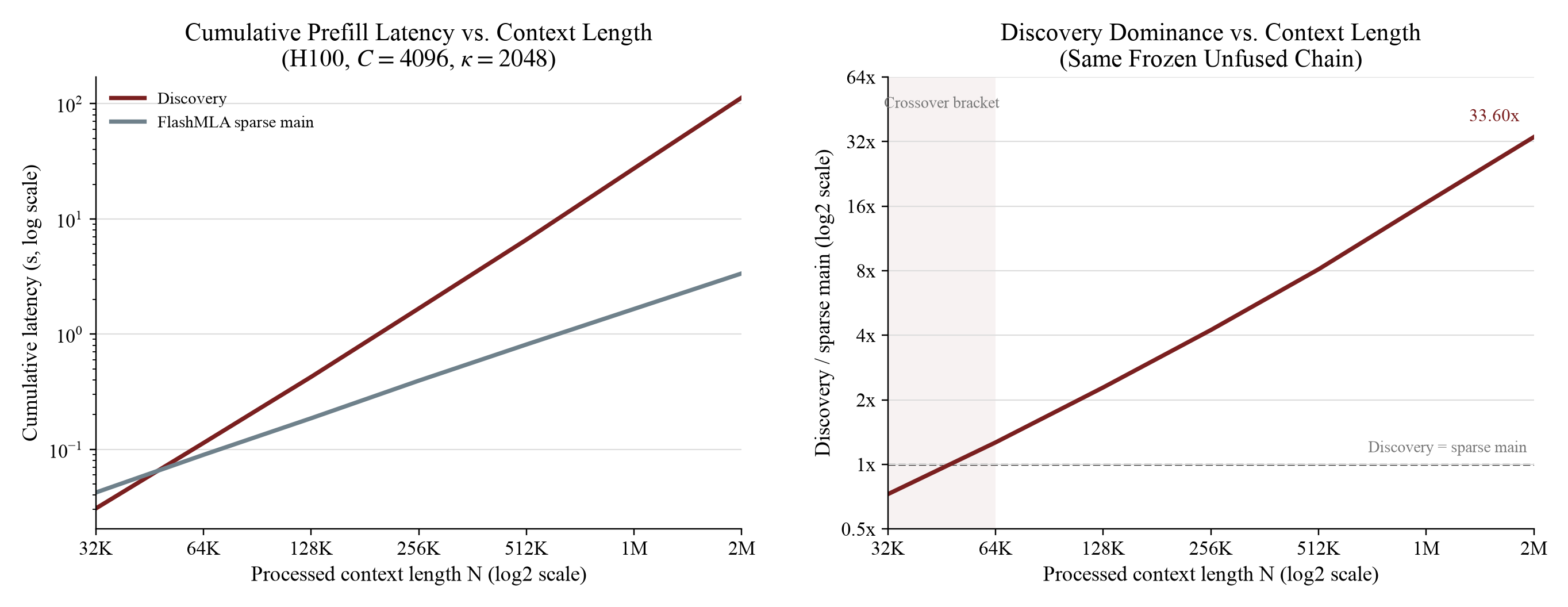
Figure 2: The left panel uses same-trial cumulative chunk-event sums from five instrumented replays, not the direct totals from 20 clean replays; the right panel plots their ratio. Checkpoints were fixed in advance and lines are visual guides. The shaded region is a discrete checkpoint bracket, not interpolation or a confidence interval.
4M is limited by capacity, so it has no latency measurement. With and the current unfused PyTorch Top-K path fixed, a strict preflight lower bound contains 64.004 GiB for the DeepGEMM carrier backing, 64 GiB for a Top-K contiguous copy, and 5.626 GiB of resident tensors:
The run was therefore marked capacity-limited before allocation. We report neither a fabricated latency nor a measured OOM. This does not mean that DSA has a universal 2M context limit: a smaller , a different Top-K implementation, or scorer–selector fusion could move the capacity boundary.
Nsys at long sequence lengths explains launch structure, not the timing curve. For one target chunk, TensorIterator splits one semantic contiguous copy inside PyTorch Top-K into approximately 1-GiB shards: eight launches at 512K and 32 at 2M. After excluding these copy shards, the Top-K kernel-family sequence and launch count remain 15, but the grids of radix, scan, gather, and related kernels grow with . It would therefore be wrong to say that the whole Top-K topology is unchanged.
In the same diagnostic captures, target-chunk attention kernel-active time changes only from at 512K to at 2M, while the discovery/attention ratio rises from to . These Nsys durations support the mechanism’s direction; they must not be spliced into the cumulative CUDA-event timing curve.
The 128K NCU data show where the traffic comes from. The 2 GiB FP32 carrier for the final query chunk at 128K causes the scorer to write approximately 1.958 GiB to DRAM in NCU; Top-K then reads 12.064 GiB— the carrier size—and writes 2.180 GiB. This traffic comes from one contiguous copy, four rounds of radix thresholding, and count, scan, gather, and related steps—not from “one read of logits and one Top-K kernel.” The Top-K stage for the 128K target chunk contains 17 CUDA kernels; the complete 4K→128K replay contains 513 Top-K kernels.
But the launch count itself is not the main loss. Across three full Nsys replays, GPU gaps inside the kernel span account for only –. Therefore, what fusion could truly eliminate is:
rather than converting the raw number of CPU launches directly into an assumed GPU speedup.
The measured facts end here. What follows is a design inference constrained by source code and resource limits, not a fused-kernel performance result. The current DeepGEMM mapping assigns two query rows to one persistent CTA, which iterates over all of their KV tiles internally. If this ownership is preserved, exact Top-2048 can be organized as online state across tiles within the CTA and does not inherently require a cross-CTA global merge. The score and ID payload alone is:
But this 32 KiB is not free. The current scorer already uses 640 threads, 96 registers/thread, and 152,228 B of dynamic shared memory, running one CTA per SM. The H100 opt-in SMEM limit is 232,448 B; after subtracting the candidate payload and approximately 4 KiB for the double-buffered score tile, only about 42 KiB of nominal space remains for merge scratch, barriers, and alignment. Inserting the selector consumer into the main loop could also cause register spills, SMEM contention, or producer backpressure, thereby degrading the existing WGMMA/TMA scorer.
The measurements therefore identify a design opportunity, not a measured speedup:
Scorer–TopK fusion may eliminate the HBM round trip for complete logits, but it does not reduce the number of candidates that an exact selector must judge, nor has it yet been shown that maintaining the selector state on chip costs less than the traffic it eliminates.
We also measured the endpoint cost of generating one new token with paged decode, up to a 4M-token history. The observed discovery/decode ratio is – from 256K through 1M, then rises to at 2M and at 4M; the direct 4M full-chain total is . These timings are not stationary: there is a clear event-latency regime shift between trials 0–4 and 5–99, and the sparse- decode event median itself drops from about at 1M to at 2M.
The 4M and earlier 128K profiles have the same visible attention launch signature— kernel identity, grid, block, and launch count—so the evidence does not explain the step as a visible dispatch change. It still cannot exclude internal branches, cache, clock, or other runtime state. We therefore use the decode data only to establish the direction of stage dominance. Neither nor any absolute latency is treated as a stable hardware constant, and the paged FP8 decode curve is not joined to the BF16 causal-prefill curve above.
5.7 Return to the Beginning: What the Two Co-design Paths Reveal
Takeaway. The algorithm decides “which data is worth accessing” and “who can share one access”; the infrastructure decides whether those accesses can be owned, rearranged, and reduced by one program. Their interface is shape, ownership, and reuse—not an abstract sparsity ratio.
Putting NSA and DSA back into one table makes their distinction more than merely block-sparse versus token-sparse:
| Question | NSA | DSA |
|---|---|---|
| Global control plane | Compression Attention at resolution | Full-token-resolution 128-D FP8 Indexer |
| Final unit of selection | Contiguous 64-token block | Arbitrary single token |
| Axis shared by the algorithm | 16 query heads in one KV group | 128 main heads |
| Where regularity appears | Before the HBM load | After discrete rows enter SMEM |
| Load reuse within one program | 16 heads | 64 heads within one SM90 head64 CTA |
| Main hidden cost | Compression path and the many-to-one reduction for | Exact all-history scan and Top-K |
Both systems have a “cheaper global scan + more expensive sparse data plane.” Keeping only the token and feature scales, NSA’s compressed sequence length is approximately:
so the number of scores in Compression Attention remains approximately:
It produces a coarse global-context output while also reusing its probabilities for selection routing. DSA’s Indexer is routing-only, but retains full token resolution, so the number of candidate scores over a complete causal sequence remains:
Neither method makes “discover globally relevant positions” asymptotically linear. Instead, each moves discovery into a cheaper representation: NSA lowers token resolution, while DSA lowers feature dimension and uses FP8. Their real difference is when regularity appears:
We must also distinguish two forms of reuse that are easy to conflate:
- semantic fanout: how many logit pairs a selection ID represents in the algorithmic semantics;
- physical load reuse: how many heads or query rows a KV row actually serves after entering a particular CTA/program.
One NSA block ID represents:
logit pairs, while the same KV row is used by 16 heads within one program. A DSA token ID is shared by 128 main heads at the algorithmic level, but the public SM90 sparse-prefill path uses two CTAs that each process 64 heads. Shared memory cannot be shared across CTAs, so the physical load reuse guaranteed within one CTA is 64, not 128. Algorithmic sharing is a necessary condition for kernel reuse, but it does not automatically equal the final reuse count of one HBM transaction.
Pipeline behavior has a similarly clear boundary. It can overlap:
metadata / indirect address
        ↓
producer or load stage
        ↓
regular on-chip tile
        ↓
dense MMA consumer
but it cannot eliminate L2 misses, TLB/page locality effects, HBM transactions, or pipeline startup and drain. Irregularity is isolated in the producer so that indirect addresses do not continue to contaminate QK, softmax, and PV; this does not turn random HBM rows into contiguous rows.
Therefore, evaluating sparse Attention requires at least the following items in one ledger:
Benchmarking only the final sparse core removes precisely the least scalable component from the chart. Likewise, explaining only how many pairs the forward pass skips—without assigning a stable owner to —does not yet produce an executable training primitive.
NSA and DSA ultimately represent two complementary but non-equivalent paths:
The real open question left by this research thread is not “what should the next sparse mask look like?” but:
Can we avoid a full selector while still exposing a sparse workload with enough sharing, regularity, and reducibility for the kernel?
Hierarchical routing, approximate retrieval, and candidate-set reuse across queries may all break the assumption of an exact all-candidate scan; but they simultaneously change model quality, dynamism, and the execution contract. The next question truly worth studying is the verifiable boundary among these three—not another isolated reduction in nominal sparsity.
Sources and Evidence
- Native Sparse Attention provides the NSA
algorithm, program mapping, and paper-reported performance results. The CSR backward
mechanism in this article was checked against the community
fla-org/flash-linear-attentionimplementation and must not be attributed to an unreleased kernel from the paper’s authors. - DeepSeek-V3.2 provides the algorithmic definition
of DSA/Lightning Indexer; the public reference logic is available in
DeepSeek-V3.2-Exp. - Code-level conclusions about the DSA scorer and sparse Attention were checked against
DeepGEMMandFlashMLA, respectively. - The causal-prefill Discovery scaling data were collected on one H100 and frozen as
Run ID
e2-h100-20260809-extended1. The body separates repeated clean timings, instrumented stage timings, capacity preflight, and profiler diagnostics; a separate 128K NCU measurement explains carrier/Top-K traffic, and profiler durations do not replace the CUDA-event curve. - The KV-row locality data were also collected on one H100 and frozen as Run ID
e3-h100-20260805-formal2. The experiment section states the conditions, paired schedule, statistical procedure, correctness checks, profiler limitations, and the boundary between synthetic indices and production traces. - The instruction semantics of Blackwell
tile::gather4follow the NVIDIA PTX ISA. This is not a path that the H100/SM90 experiments in this article can validate. - The organization of this article draws on MLA, dim by dim and its Chinese version: state the conclusions first, then derive them dimension by dimension through a unified tensor lens. This article follows the same method further into program ownership, memory movement, and backward reduction.