
Profiling Ozaki II: Why Can Preprocessing Cost More Than Matrix Multiplication?
Oct 1, 2026
TL;DR
- Ozaki II replaces one slower double precision matrix multiplication (FP64) with several very fast integer matrix multiplications (INT8). With the main multiplication already handled by INT8 Tensor Cores, preparing the inputs instead becomes more time-consuming, in many cases approaching or even exceeding the main GEMMs. This article investigates why.
- Most preprocessing time goes into generating multiple sets of integer residues. To prepare high precision inputs for multiple INT8 matrix multiplications, every input element must be reduced repeatedly under different moduli. In the large-matrix, many-modulus configurations we tested, this step accounts for most preprocessing time.
- Generating INT8 residues still incurs the cost of FP64 arithmetic. Source and assembly show several floating point instructions per residue, while H20 hardware metrics show the ordinary FP64 execution path used by preprocessing approaching saturation. The main GEMMs use much higher throughput INT8 Tensor Cores. Preprocessing can therefore do less arithmetic yet take a comparable amount of time, or even longer.
- Further acceleration requires attention to the cost of preparing inputs. As the main GEMMs become faster, preprocessing becomes harder to ignore in the total runtime. Our analysis points to a concrete optimization direction: reduce the FP64 work needed to generate the INT8 inputs while preserving correct residues, then evaluate the benefit using the complete computation’s runtime.
Part I Goal: Emulating high precision matrix multiplication with high throughput low precision matrix multiplication
1 Computing a high precision product with multiple INT8 GEMMs
Let , , and . Each output is a dot product of length ; in the square experiments, . Ozaki II chooses small, pairwise coprime moduli , with product , and jointly represents scaled integer inputs through their residues.[1]
Product bounds first determine diagonal scaling matrices and , whose diagonal entries are positive powers of two. Left multiplication by scales rows of A; right multiplication by scales columns of B. The complete pipeline follows, with identifying the modulus channels:
| Stage | Operations and formulas | Color used below |
|---|---|---|
| Input preprocessing | Estimate bounds and choose , then scale and truncate toward zero: , . Generate INT8 residues: , . | Green |
| Main matrix multiplication | , using INT8 × INT8 → INT32 GEMM. | Yellow |
| Output reduction | , taking a nonnegative residue for each entry. | Blue |
| Combination and inverse scaling | Combine residue channels: . Restore the original scale: . | Red |
Here takes centered residues entrywise. The operator reconstructs each entry in using the Chinese Remainder Theorem. Scaling must ensure , so exact arithmetic would reconstruct . We denote the final approximation by , since integerizing the inputs and performing reconstruction can still introduce error.
Exact computation in the low precision core depends on two range conditions. Each modulus is at most 256, allowing centered residues to fit into signed INT8’s . Each product has magnitude at most , so
is sufficient to prevent INT32 accumulation overflow, including intermediate partial sums. Integer multiply-accumulate operations within range are exact. Accuracy of the complete FP64 result still depends on input truncation and reconstruction. Paper, Section 3.1[1]
Using moduli requires main GEMMs. More moduli enlarge the reconstruction range and generally allow more input information to be retained, at the cost of additional input residues, GEMMs, and output processing. The suffix 14 in fast-14 and accu-14 denotes 14 moduli for the main computation.
2 How fast and accu trade bound estimation cost for accuracy
Scaling balances two requirements: amplify inputs enough to limit information lost during integerization, while keeping the integer product inside the reconstruction range. This requires an upper bound on each output’s magnitude before performing the main multiplication.
Fast estimates the bound from row and column norms. Cauchy–Schwarz gives
Scanning rows of A and columns of B takes work. The bound discards matching positions: both norms can be large even when their large entries occur at different positions, making the scaling unnecessarily conservative.
Accu estimates the bound with one additional INT8 GEMM. It scales and rounds absolute inputs upward into INT8 matrices, ensuring that each reconstructed entry bounds the original absolute value. Their product then supplies a bound that retains positional relationships. This can reduce overestimation and preserve more input information under the same modulus budget, although the effect depends on the data and quantization.
For the performance discussion, the location of this extra work matters: accu’s bound-input conversion, bound GEMM, and output reduction all belong to green preprocessing. Green therefore includes an matrix multiplication in accu, alongside its elementwise operations. The paper’s two bounds[1]
3 Once the main multiplication is faster, preprocessing becomes a substantial cost
The paper compares against native DGEMM, or double precision matrix multiplication, in NVIDIA’s cuBLAS matrix library. The table below selects representative results from two GPUs, measured in effective TFLOPS: the final task’s operations divided by total elapsed time, rather than the internal work of all GEMMs.
| GPU / matrix order | Native DGEMM | fast-14 | accu-14 | fast-18 | accu-18 |
|---|---|---|---|---|---|
| GH200 / 16384 | 60.9 | 80.2 | 71.1 | 62.6 | 56.6 |
| RTX 4090 / 8192 | 0.62 | 9.81 | 9.23 | 7.83 | 7.41 |
Source: the paper’s GPU throughput measurements (Tables 3 and 4[1]). All sizes and modulus configurations are retained in the supplement.
Fast-14 reaches approximately 1.32× and 15.8× the throughput of native DGEMM in these two configurations. The difference is related to hardware throughput ratios: the paper lists dense INT8 Tensor / FP64 Tensor peaks of 1979 TOPS / 67 TFLOPS for GH200, while RTX 4090 has INT8 Tensor / ordinary FP64 peaks of 660.6 TOPS / 1.29 TFLOPS. RTX 4090 has much weaker native FP64 throughput than GH200. Paper hardware specifications[1] In addition, fast is consistently faster than accu at the same size and modulus count, and increasing the number of moduli lowers throughput.
Next, consider the stage fractions for two large-matrix configurations:
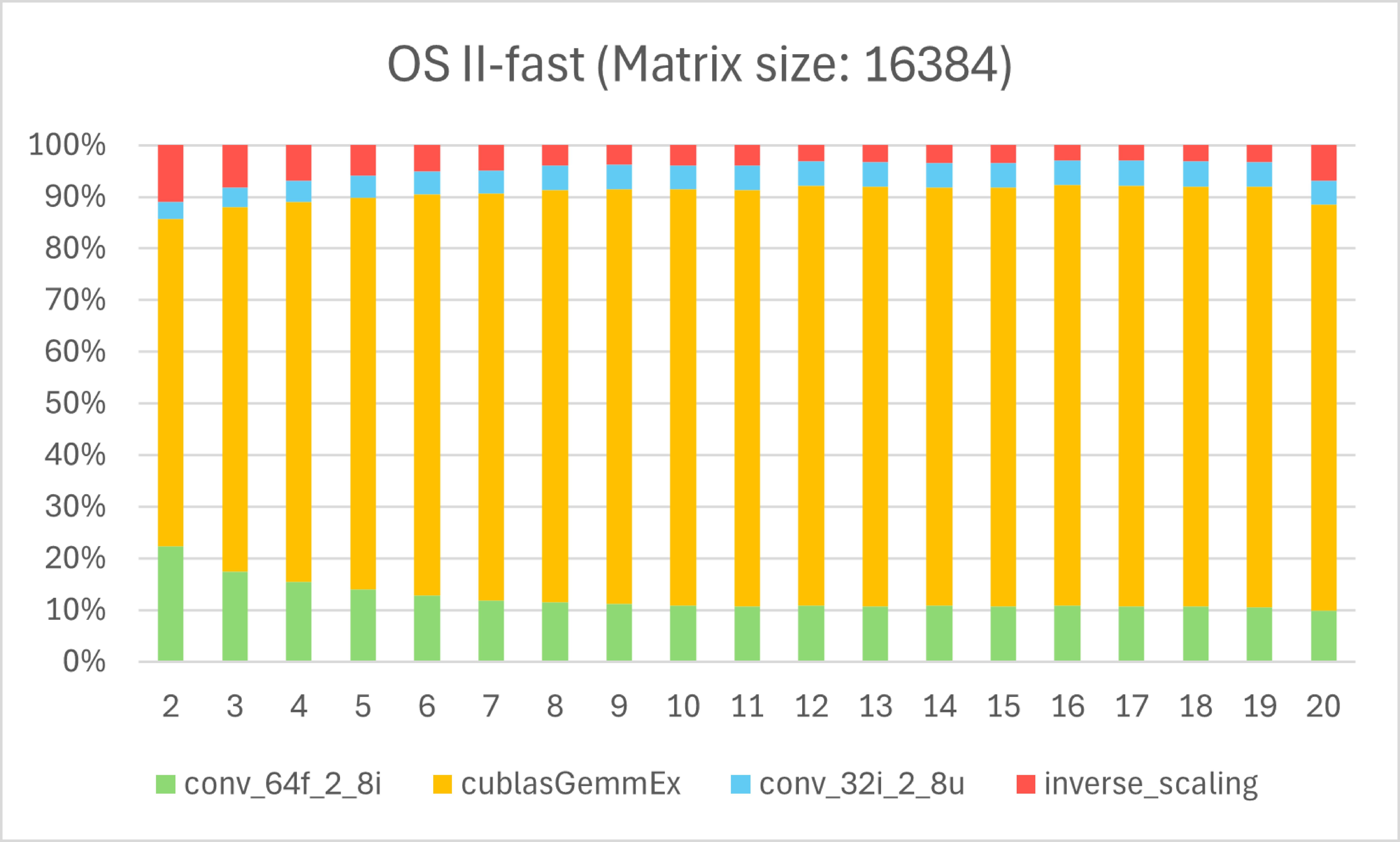
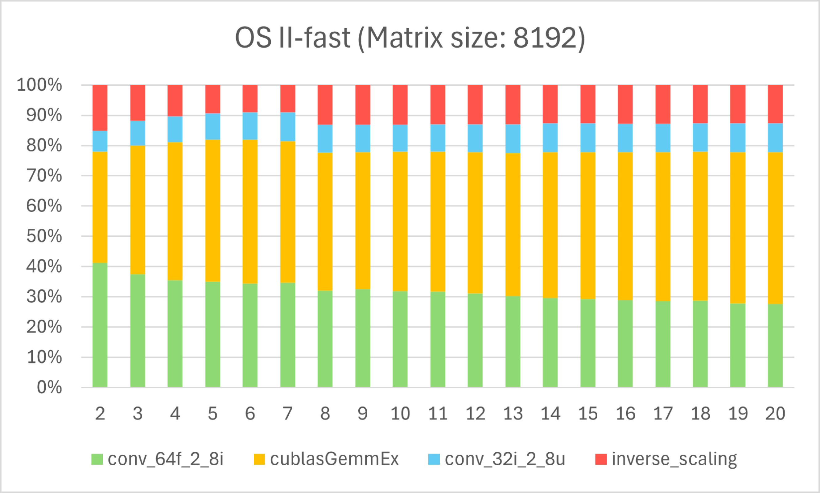
GH200 is on the left and RTX 4090 on the right; narrow screens stack them vertically. The horizontal axis is the modulus count, each bar is normalized to 100%, and the colors follow the pipeline table in Section 1. Excerpts from paper Figures 6(d) and 7(d)[1]. The two figures use different matrix sizes and show relative rather than absolute speed.
The figures show that the main GEMM share generally increases with matrix size. Yet even when the main GEMMs (yellow) account for most of the time, preprocessing (green) remains a substantial cost. We investigated this in detail using profiling tools on H20: first measuring elapsed time, then examining complexity, hardware counters, and machine instructions to explain the results step by step.
Part II Reflections: Further profiling analysis of the Ozaki II method
4 Reproduction experiments on H20-3e
Our first step is to establish the timings: how much does preprocessing (green) cost, and at which sizes and configurations does it approach or exceed the main GEMMs (yellow)? We then trace the operations and hardware costs behind it.
We ran the reproduction on a single H20-3e, testing four square matrix sizes, , both bound-estimation modes (fast and accu), and modulus counts . Each configuration used 3 warmups and 30 measurements. Inputs followed the historical code’s generator, with and seed=123456; A and B used the same seed.
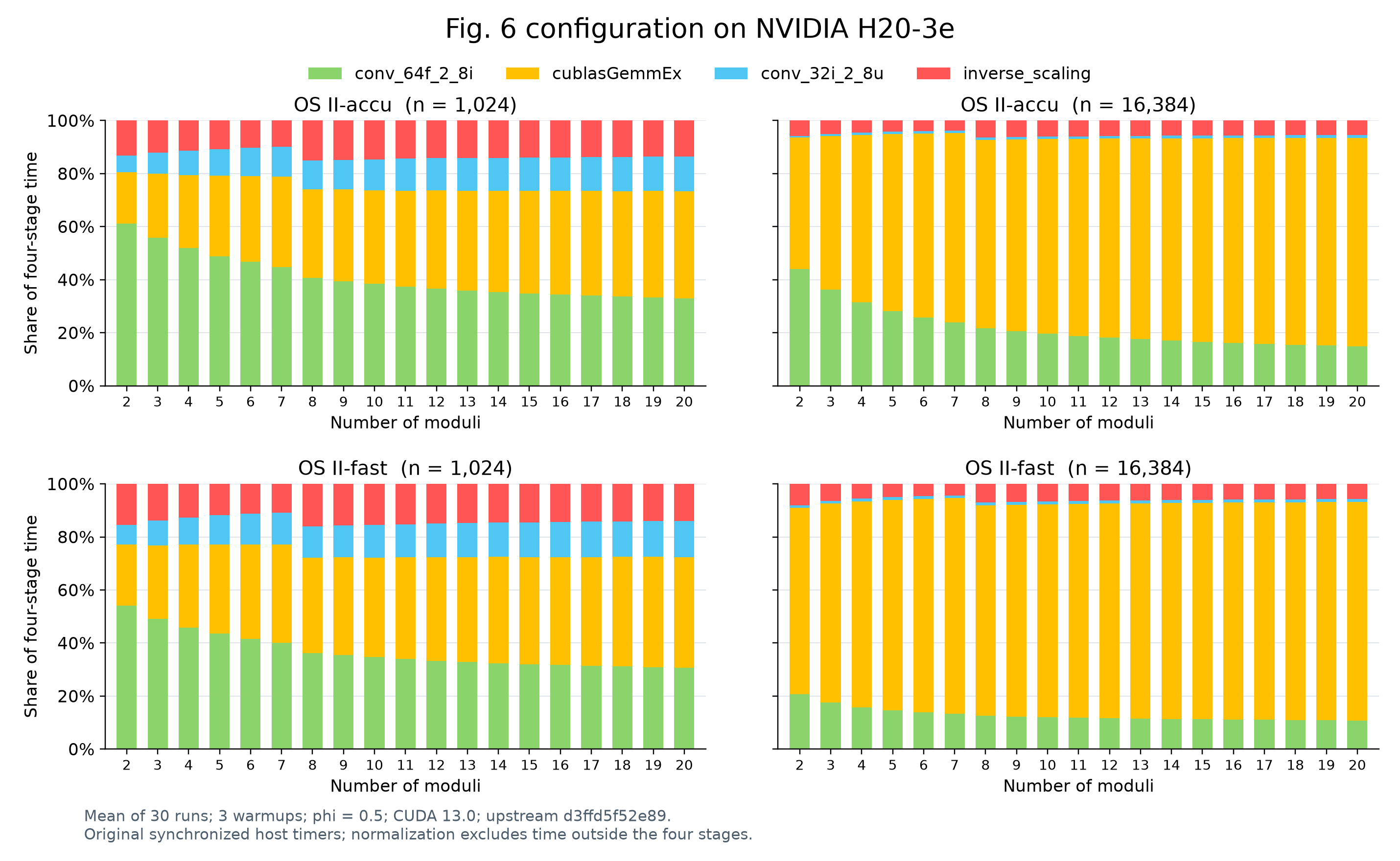
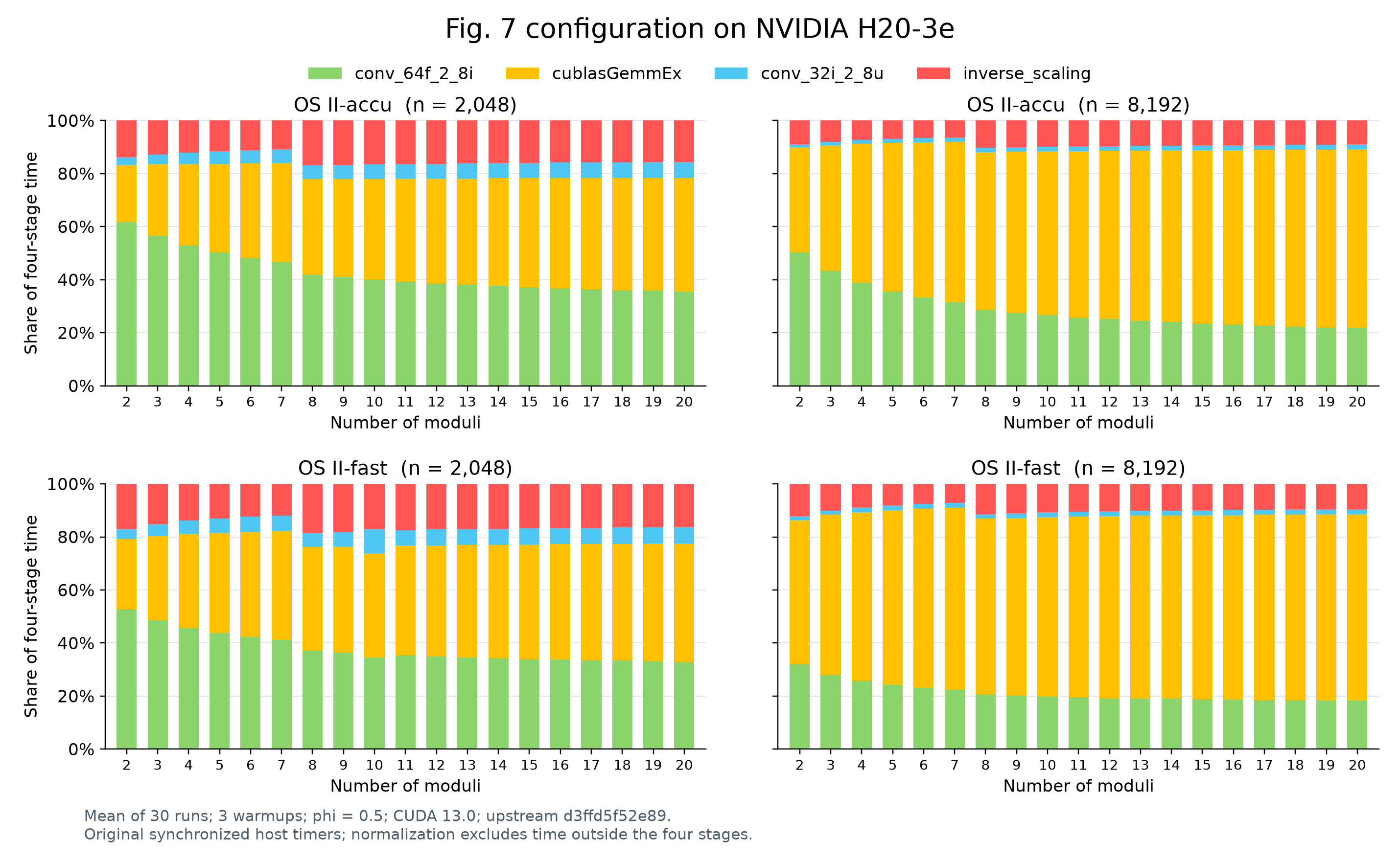
Stage fractions measured on H20-3e. The first plot follows the matrix-size layout of paper Figure 6, and the second follows Figure 7; both use our reproduction data rather than the original paper results.
First, consider several absolute timings and ratios for fast:
| Green ms | Yellow ms | Green / yellow | Yellow INT8 TOPS | ||
|---|---|---|---|---|---|
| 1024 | 2 | 0.1267 | 0.05394 | 2.35 | 79.6 |
| 2048 | 14 | 1.0554 | 1.3161 | 0.802 | 182.8 |
| 8192 | 14 | 15.3937 | 55.9376 | 0.275 | 275.2 |
| 16384 | 14 | 60.5876 | 436.3535 | 0.139 | 282.2 |
In many configurations, such as size 2048 with 14 moduli, preprocessing costs almost as much as all the main GEMMs combined. Even at size 8192, green remains 27.5% of yellow. This is the observation we need to explain.
5 Timing measurements: input preprocessing
5.1 Input statistics determine the scaling
The fast path scans each row of A and column of B for a maximum absolute value and a sum of squares. Warp shuffles, shared memory, and block reductions combine these values; the kernel then computes a power-of-two scaling exponent.
These statistics are part of the numerical method. The sum of squares supports the norm-related bound, and the maximum and exponents participate in scaling. They are not logging or a simple average. Upward rounding in the sum of squares and additions helps avoid underestimating the bound.
The original implementation fuses statistics, scaling, truncation, and residues into two GPU kernels, one for A and one for B. A kernel is a function executed collectively by many GPU threads; one launch can contain several different operations.
fast
  A row statistics → scale exponent → scale/truncate → s residues
  B column statistics → scale exponent → scale/truncate → s residues

accu
  Upward quantization of |A| and |B| → one bound GEMM
  Row/column maxima of the bound output → final scale exponents
  Scale/truncate original A and B → s residues
Note: Input generation, workspace allocation, and host-to-device transfers are outside our green timings. Historical
scaling.hpp[2]
5.2 A detailed timing breakdown of preprocessing
We added a diagnostic version that separates the final fused kernel into statistics, scale/truncate, and residue generation. It retains the original access directions and thread mapping, storing intermediate integer-valued data in FP64 arrays. All INT8 residues and scaling exponents matched the original implementation across all 12 validation groups: three sizes, two modes, and two diagnostic variants.
At , combining A and B timings gives:
| Diagnostic stage | fast ms | fast share | accu ms | accu share |
|---|---|---|---|---|
| Prepare bound INT8 inputs | — | — | 2.486 | 11.6% |
| Bound GEMM | — | — | 4.034 | 18.8% |
| Statistics and final scaling choice | 1.239 | 8.0% | 0.656 | 3.1% |
| Scale, truncate, and write intermediate data | 1.937 | 12.5% | 1.936 | 9.0% |
| Generate and write residue channels | 12.330 | 79.5% | 12.330 | 57.5% |
| Total | 15.506 | 100% | 21.442 | 100% |
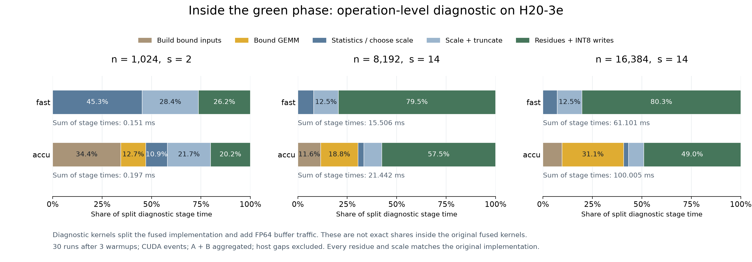
Stage shares in the split diagnostic.
Note: Splitting adds intermediate FP64 reads and writes, kernel launches, and changes to register and cache behavior. At size 8192, total device time increases by about 0.7% for fast and 3.3% for accu; at size 1024 with two moduli, the disturbance is about 19%. These results nevertheless identify the largest component: with many moduli and large matrices, residue generation occupies most of fast preprocessing. However, in the split result at size 1024 with two moduli, statistics account for about 45.3%, scaling 28.4%, and residues 26.2%; fixed scanning costs are more prominent.
The accu path also performs a GEMM during preprocessing to estimate the bound (yellow in the operation-breakdown figure). This extra GEMM becomes more prominent as the matrix grows. CUDA event measurements put it at about 19.5% of preprocessing at size 8192, rising to about 32.0% at size 16384.
6 Complexity analysis: how matrix size and modulus count affect execution time
Counting serial work and ignoring the constant costs of fixed precision arithmetic, we obtain the following estimates:
| Operation | General shape | Square case |
|---|---|---|
| fast input statistics | ||
| Scaling and truncation | ||
| Input residues | ||
| accu bound input conversion | ||
| accu bound GEMM | ||
| accu bound output reductions | ||
| Yellow main GEMMs | ||
| Blue output residues | ||
| Red CRT and inverse scaling |
Note: The last row assumes this implementation’s fixed one-word or two-word working precision. If target precision grows without bound, the cost of multiprecision arithmetic must also be included.
Thus fast’s green work is approximately , while accu adds an term. Holding and doubling size from 8192 to 16384 increases measured fast green time by 3.94×, yellow by 7.80×, and accu green by 4.70×. These are consistent with quadratic, cubic, and mixed growth.
At fixed , linear fits over give
The slopes are almost identical, while accu has a larger intercept, reflecting additional bound-estimation work independent of . This means that each extra modulus adds almost the same preprocessing time to fast and accu, but accu also pays an additional bound-estimation cost.
After analyzing complexity, the question becomes: why does preprocessing take about as long as the main GEMMs? Hardware and other constraints mean that algorithmic complexity cannot be equated directly with elapsed time. We therefore need to examine the actual hardware execution to investigate further.
7 Kernel analysis: identifying what limits preprocessing
Nsight Compute (NCU below) is NVIDIA’s GPU kernel analysis tool, which exposes hardware metrics for execution pipelines and memory systems.[4] DRAM throughput in the table refers to the transfer rate of GPU memory. We sampled the original, unsplit fast kernels with it:
| Kernel | FP64 pipeline % | INT Tensor pipeline % | DRAM throughput % | |
|---|---|---|---|---|
| 1024/2 | Green A | 88.1 | 0 | 1.13 |
| 1024/2 | Green B | 89.3 | 0 | 0.62 |
| 2048/14 | Green A | 95.6 | 0 | 3.62 |
| 2048/14 | Green B | 95.8 | 0 | 3.46 |
| 2048/14 | Yellow GEMM | 0 | 73.4 | 2.56 |
| 8192/14 | Green A | 98.0 | 0 | 5.04 |
| 8192/14 | Green B | 98.3 | 0 | 4.88 |
| 8192/14 | Yellow GEMM | 0 | 95.4 | 9.79 |
Note: Each column is normalized to the sustained peak of its corresponding resource.[4]
The key to interpreting these numbers is that ordinary FP64 CUDA Core arithmetic on H20 has much lower throughput than INT8 Tensor Core matrix multiplication. Here, ordinary FP64 CUDA Cores means the SM units that execute per-thread double precision arithmetic. Green’s approximately 98% FP64 metric indicates that this execution path is already busy; yellow’s approximately 95.4% INT Tensor metric indicates heavy use of its matrix resources. Similar percentages refer to very different throughput ceilings, so they do not imply similar absolute operation rates.
Green is approaching the capacity of a relatively low throughput FP64 path, while yellow runs on a much higher throughput INT8 Tensor Core path. Even when both use their respective resources efficiently, green can take a comparable amount of time, or longer, because each unit of its work is more expensive to execute. This comparison concerns aggregate parallel throughput, rather than the latency of an individual FP64 instruction versus a Tensor instruction.
A is read by rows from column-major storage, producing strided accesses, while B’s column reads are more contiguous. Yet A and B have similar times and both heavily use the FP64 pipeline. Along with low DRAM and cache throughput metrics, this supports FP64 execution throughput as the primary limitation in these samples. Strided access remains an optimization candidate, but its presence in source code does not establish a bandwidth bottleneck.
We can understand the functional organization inside an SM as follows:
SM schedulers and registers
    ├── Ordinary FP64 CUDA Core path: per-thread arithmetic, lower throughput
    ├── INT8 Tensor Core path: cooperative matrix multiply-accumulate, high throughput
    └── Memory, conversion, and other execution paths
The throughput gap reflects different compute structures and hardware resource allocations. Ordinary FP64 arithmetic handles a wide significand, exponents, normalization, and rounding. INT8 Tensor Cores use narrow integer arithmetic and dedicated matrix structures to execute many operations per cycle while reusing operands. This lets them process GEMM’s large multiply-accumulate workload at high throughput. NVIDIA’s description of Hopper Tensor Cores[3]
Writing an INT8 output does not make the preceding computation suitable for INT8 Tensor Cores. Remainder generation, rounding, and maximum reductions do not directly have a matrix multiply-accumulate structure. Many GPU threads still execute these elementwise operations in parallel, but their combined rate is limited by the relevant resources.
The complexity comparison in Section 6 therefore needs the hardware execution rates: fast preprocessing performs mainly work, but its repeated FP64 operations use the lower throughput path. The main GEMMs perform work on much higher throughput INT8 Tensor Cores. This explains how preprocessing can do less work and still remain expensive. The next section examines source and assembly to identify the FP64 operations required to produce each INT8 residue.
8 Which instructions does one INT8 residue require?
Section 7 identifies ordinary FP64 execution throughput as a constraint on preprocessing. We now need to trace the source of that FP64 work: why does preparing INT8 residues keep double precision execution resources so busy?
The breakdown in Section 5 points to residue generation. We follow one input element under one modulus, examining the function’s inputs and outputs, its numerical steps, and the actual machine instructions. We then scale that cost up to the full matrices.
8.1 Taking the remainder of an FP64 value
Before the remainder function is called, each original element has been scaled by a power of two and truncated toward zero. It is mathematically integer-valued, but the program still stores it in a double. Call this value , and the current modulus . We need a small integer congruent to modulo , suitable for the subsequent INT8 GEMM.
Subtracting an integer multiple of the modulus moves the value toward zero:
An accurately computed nearest integer quotient would leave a residual within roughly half the modulus. The implementation challenge is that and its quotient can be large while the desired remainder is small. Preserving low-order information when subtracting large values therefore matters directly to correctness.
The historical implementation contains:
const auto val = oz2_table::moduli_dev[j];
float tmp = __double2float_rn(fma(rint(a * val.y), val.x, a));
tmp = __fmaf_rn(rintf(tmp * val.w), val.z, tmp);
tmp = __fmaf_rn(rintf(tmp * val.w), val.z, tmp);
return static_cast<int8_t>(tmp);
The four constant-table fields have the following meanings:
| Field | Type | Meaning |
|---|---|---|
val.x | FP64 | |
val.y | FP64 | Precomputed approximate reciprocal |
val.z | FP32 | |
val.w | FP32 | Precomputed approximate reciprocal |
The reciprocals are stored in GPU constant memory, allowing each reduction to estimate the quotient through multiplication. See mod_8i<double> and the modulus table[2].
8.2 Three reduction passes for remainder calculation and correction
First pass: use FP64 to remove most of the modulus multiples in the input.
The first arithmetic line expands into:
Here and round to the corresponding floating point formats. rint rounds to a nearest integer, with ties to even, while retaining a floating point return type. The steps estimate an integer quotient, compute the remaining part, and convert that smaller residual to FP32.
The FMA matters: fma(h0, -m, a) computes as one fused operation, rounding only the final result. Rounding the large intermediate product separately before subtracting it from could discard low-order information needed for the small remainder. CUDA definitions of rint and fma[6]
FMA controls rounding within the multiply-add. It does not make the estimated quotient exact: the approximate reciprocal and rounding of can still move away from the ideal nearest integer quotient. The first residual can therefore retain additional multiples of the modulus.
Second and third passes: apply FP32 corrections to the smaller residual.
The two __fmaf_rn lines perform the same operation, with the second consuming the tmp updated by the first:
Each pass estimates how many additional modulus multiples should be removed to move the current residual toward zero, then subtracts that integer multiple using FMA. The initial FP64 pass has substantially reduced the magnitude, allowing subsequent reduction to operate on smaller values. This explains the mixed precision structure: start in FP64, then correct in FP32.
Finally, is converted to the INT8 output. The complete path is:
Scaled, truncated FP64 input
    → FP64 quotient estimate and fused subtraction of modulus multiples
    → Convert to FP32
    → FP32 quotient estimate and correction, twice
    → Convert and pack into INT8
An eight-bit result does not imply that eight-bit intermediate arithmetic is sufficient. Converting the large original to FP32 first can change its residue through rounding; later corrections cannot automatically recover lost information. This implementation handles the large value before reducing the precision used for the residual. Floating point rounding semantics of rintf[6]
8.3 Mapping every step to actual machine instructions
Source establishes the numerical steps; compiled instructions establish the work they actually produce. SASS is NVIDIA’s machine instruction representation. We inspect the SM90 code in the original experiment’s gemmul8.o:
cuobjdump --dump-sass build/gemmul8.oThe table follows one element’s data dependencies in vecnorm::scalingB_kernel<double>. Names such as R16 and R32 identify registers; an FP64 value occupies two adjacent 32-bit registers. Addresses are nonconsecutive because the compiler interleaves operations for other elements.
| Address | Actual instruction | Corresponding computation |
|---|---|---|
1780 | DMUL R32, R16, R24.reuse | Multiply by the reciprocal in FP64 to estimate |
17d0 | FRND.F64 R32, R32 | Round the approximate quotient to floating point integer |
1800 | DFMA R32, R32, R22, R16 | Compute with an FP64 FMA |
1830 | F2F.F32.F64 R27, R32 | Convert the residual to FP32, producing |
1890 | FMUL R36, R23.reuse, R27 | Estimate in FP32 |
18c0 | FRND R36, R36 | Obtain the integer quotient for the first FP32 correction |
18f0 | FFMA R27, R22, R36, R27 | Compute corrected residual |
1910 | FMUL R30, R23, R27 | Estimate from the updated residual |
1920 | FRND R30, R30 | Obtain the second correction quotient |
1960 | FFMA R27, R22, R30, R27 | Compute |
1980 | F2I.TRUNC.NTZ R26, R27 | Convert to an integer register value for subsequent INT8 packing |
The D in DMUL and DFMA denotes double precision multiply and fused multiply-add; FMUL and FFMA operate in single precision here. FRND rounds a floating point number to an integer value, F2F changes floating point format, and F2I converts to an integer representation. Subsequent PRMT byte packing and stores remain, so the table’s last row is not the end of preprocessing. NVIDIA instruction classifications[5]
This element’s chain contains one FP64 multiplication, one FP64 rounding, one FP64 FMA, one FP64-to-FP32 conversion, two groups of three FP32 correction instructions, and an integer conversion. It also has dependencies: the FP32 corrections need the FP64 residual, and the second correction needs the first correction’s result.
Interleaving elements hides some waiting, and additional threads supply parallel work. Neither removes the arithmetic demand per residue. Once the constrained execution path is already busy, additional parallelism cannot increase throughput indefinitely. Exact pipeline attribution still requires counters; instruction mnemonics alone do not assign all of this work to the FP64 metric.
This was a read-only inspection of the original object, without another GPU performance run.
8.4 How many times does this chain repeat?
The enclosing kernel scales and truncates an element before repeatedly calling mod_8i inside its modulus loop. The code handles four elements at a time and calls the function separately on all four values, producing four elementwise reduction chains.
For two input matrices and moduli, the valid inputs require
residues. At , this is 1,879,048,192 residues, or about 1.879 billion. Expanded per valid element, this work alone requires approximately 1.879 billion FP64 multiplications and the same number of FP64 FMAs, plus rounding, FP32 corrections, conversions, and writes.
These are operation demands summed over elements. GPU instructions are issued at granularities such as warps, with one instruction serving multiple threads. The counts are therefore not hardware instruction issue counts, and multiplying the table’s 11 rows by the residue count would not establish the whole kernel’s dynamic instruction count.
Other green operations also use FP64. In input statistics, DFMA.RP and DADD.RP implement upward-rounded sum-of-squares accumulation and reductions. Scaling and truncation generate additional instructions. The high FP64 metric in Section 7 reflects the combined demand of the original fused kernel. Section 5’s diagnostic timing further identifies repeated residue generation as its largest time component in this large-matrix, many-modulus configuration.
8.5 Comparing the main GEMM execution path
The main GEMMs receive INT8 matrices that have already been prepared. They can perform matrix tile multiply-accumulates directly, without repeating the reduction chain for each multiply-add. Nsight Systems recorded this cuBLAS kernel at matrix order 8192:
sm90_xmma_gemm_i8i32_i8i32_i32_tn_n_tilesize256x128x128_
warpgroupsize2x1x1_execute_segment_k_off_kernel__5x_cublas
Its INT8/INT32 matrix kernel identity agrees with NCU’s approximately 95.4% INT Tensor metric. Runtime identity and counters establish the main GEMM Tensor Core path; we did not export the full dynamically linked cuBLAS disassembly.
The cost is now concrete: every input element under every modulus requires a reduction chain containing FP64 arithmetic, while the main GEMMs perform large numbers of multiply-adds on prepared residues at INT8 Tensor Core throughput. The next section combines work counts and actual processing rates to check whether they explain the measured time ratio.
9 Why less arithmetic can still take more time
9.1 Which measurement does 22% describe?
Every time ratio in this section uses the yellow main GEMMs as its denominator. For example, 22% means that residue generation takes 22% of the GEMM time, not 22% of the complete stacked bar.
For square matrices, input conversion generates
residues, while the main products execute
integer multiply-adds. Their count ratio is . If each unit of work had the same cost, GEMM would clearly dominate.
Define as residues generated per second and as integer multiply-adds per second. By these definitions of effective rates,
At size 8192 with 14 moduli:
| Work | Count | Time | Effective rate |
|---|---|---|---|
| Residue generation | Approximately 1.879 billion | 12.330 ms | Approximately 152.4 G residues/s |
| INT8 multiply-adds | Approximately 7.697 trillion | 55.938 ms | Approximately 137.6 T multiply-adds/s |
There are 4096 times as many multiply-adds, but their effective processing rate is approximately 903 times higher. Residue generation can therefore still take
of the yellow time.
The 22% is a reformulation of the size-8192, 14-modulus measurements, not a theoretical expectation for other configurations. The factor 903 comes from measured effective rates; it is neither a fixed hardware peak ratio nor the latency ratio of two instructions. Computing rates from measured times and substituting them back into the equation does not produce an independent prediction. It explains how a rate difference offsets a work-count difference. The preceding timing breakdown, counters, and assembly supply the evidence for the underlying cause.
9.2 Why is complete preprocessing 27.5% rather than 22%?
The 22% covers residue generation only. Fast preprocessing also includes statistics, scaling, and truncation. The same split diagnostic measured 1.239 ms and 1.937 ms for those additional stages, giving
The original fused preprocessing instead gives
These are close but unequal because splitting adds intermediate memory traffic and kernel launches and changes execution behavior. Diagnostic and original stage timers also have different boundaries. This reconciles the magnitudes; it is not an exact allocation of time within the original fused kernel.
9.3 Why can other configurations at the same size greatly exceed 27.5%?
First change only the modulus count. Section 6 fitted preprocessing at size 8192 as
Each main GEMM takes approximately 4 ms in these measurements, so ms. Consequently,
The first term is the preprocessing work that grows with modulus count, relative to the main GEMMs: about 22% in these data. The second term comes from work approximately independent of modulus count, amortized over the yellow GEMMs. With fewer moduli, this cost becomes more prominent relative to yellow. Here, “fixed” means approximately independent of at a given matrix size; it does not mean independent of matrix size.
| Moduli | Fast fitted ratio | Fast measured ratio | Accu fitted ratio | Accu measured ratio |
|---|---|---|---|---|
| 2 | 59.7% | 59.3% | 126.1% | 126.3% |
| 14 | 27.5% | 27.5% | 37.0% | 37.0% |
| 20 | 25.9% | 25.9% | 32.6% | 32.3% |
All rows use size 8192. The fit reuses the same measurements to explain their variation; it is not an additional predictive validation.
For fast with 14 moduli, the approximately 3 ms of work independent of modulus count is only about 5.4% of the approximately 56 ms yellow time. With two moduli, it is about 37.6% of the approximately 8 ms yellow time. Adding the work that grows with modulus count raises green/yellow from approximately 27.5% to 59.3%.
Accu additionally prepares bound-estimation inputs, executes a bound GEMM, and processes the bounds, increasing its cost independent of . With two moduli, this is enough to make complete preprocessing exceed the main GEMMs. The measured 126.3% is therefore consistent with this cost structure.
9.4 Smaller matrices change both work ratios and effective rates
Changing matrix size at a fixed modulus count also changes the expected ratio. The work-count ratio is : 4096 at size 8192, 1024 at size 2048, and only 512 at size 1024. As matrices shrink, the cubic GEMM work decreases relative to quadratic preprocessing. At approximately stable effective rates, residue/yellow and fast green/yellow therefore increase roughly as .
Measured fast ratios at a fixed are:
| Matrix size | Green/yellow |
|---|---|
| 1024 | 80.6% |
| 2048 | 80.2% |
| 8192 | 27.5% |
| 16384 | 13.9% |
The ratio nearly halves from 8192 to 16384, but is almost unchanged between 1024 and 2048. Small configurations therefore do not follow a constant-rate approximation. Effective throughput on both sides changes with size, work per thread, kernel selection, and launch and synchronization costs. For example, yellow reaches only about 79.6 INT8 TOPS at size 1024 with two moduli, versus about 275.2 TOPS at size 8192 with 14 moduli. The rate ratio 903 cannot be transferred between them. Slower GEMMs by themselves lengthen yellow and reduce green/yellow; a high ratio on a small matrix cannot simply be attributed to low Tensor Core utilization.
Statistics and scaling are also particularly important for small matrices with few moduli. At size 1024 with two moduli, fast split diagnostics attribute about 45.3% of green to statistics, 28.4% to scaling, and only 26.2% to residue generation. Original green/yellow reaches 234.9%, with a substantially different cost composition from size 8192 with 14 moduli. Splitting also causes a larger disturbance in this small configuration, so these diagnostic shares identify major operations but should not be multiplied into original timings as an exact decomposition.
For accu, both the extra bound GEMM and the main GEMMs grow as . At fixed , increasing cannot amortize that extra product in the same way as quadratic preprocessing.
When comparing other bars, check whether the numerator covers residues or complete preprocessing, whether modulus count and matrix size match, and whether accu’s additional bound estimation is included. Both 22% and 27.5% have specific configurations and timing scopes. Higher or lower ratios elsewhere follow from changes in this work and its effective execution rates.
10 Implications for further optimization
The preceding evidence narrows the first place to change down to mod_8i<double>: in the diagnostic with large matrices and many moduli, residue generation accounts for about 80% of fast preprocessing. It repeats an FP64 multiplication and FMA for every element and every modulus, while the FP64 pipelines of the original preprocessing kernels are already nearly saturated. Below are some ideas that I think may be worth trying.
10.1 Convert each element to an integer representation once, then generate its residues
The current code already scales and truncates each element outside the modulus loop and reuses it in registers across the residue calculations. Since the scaled value is already integral, we can perform one exact integer conversion outside the loop and use primarily integer arithmetic inside it.
We can try this for finite scaled values satisfying . Within this range, an integer-valued FP64 number can be converted exactly to INT64; outside the range, retain the original remainder path. CUDA provides the corresponding __double2ll_rz conversion, but the range must be checked before converting. NVIDIA conversion documentation[6]
One concrete approach splits the magnitude into high and low unsigned 32-bit integers:
Perform the split once. For each fixed modulus , precompute , then use
to generate the residue. Finally, handle the original sign and map the result to the signed residue required for INT8. Since , after reducing the high and low parts separately, the expression in brackets is at most , so the combination can use 32-bit integer arithmetic. For , the result must also stay within the INT8 range.
The moduli come from a fixed table, so specialized code can be generated for each modulus to implement these remainders with fixed-divisor integer reductions. Inspect whether the compiler lowers them to instructions such as multiply-high, shifts, and corrections. Directly replacing floating point reduction with a general runtime INT64 % does not guarantee a speedup. Keep conversion, splitting, and range checks in the original fused kernel where possible, avoiding an additional full INT64 intermediate matrix written to memory.
This changes the work arrangement to:
Current:   scale/truncate once → FP64 initial reduction and FP32 corrections for each modulus
Prototype: scale/truncate once → convert/split once → integer reduction for each modulus
It targets the repeated FP64 cost identified earlier.
10.2 Group moduli to overlap input preparation and the main GEMMs
Once the remainder implementation is stable, we can try preparing inputs for a small group of moduli at a time. Record an event when preparation finishes, then let the compute stream run the corresponding GEMMs while the preparation stream generates the next group’s inputs. Alternate between two input buffers, overwriting each only after the GEMMs consuming it have finished. Retain the output residues from all channels for subsequent CRT reconstruction.
Preparation: group 0 inputs → group 1 inputs → group 2 inputs
Compute:                     group 0 GEMMs → group 1 GEMMs → group 2 GEMMs
This experiment tries to hide some of the preprocessing time. It requires removing stage synchronizations that prevent overlap and avoiding repeated input statistics for each group. Grouping may increase input reads and kernel launches. FP64 and Tensor Core operations also share resources such as SMs and registers, so experiments are needed to determine whether the change actually improves performance.
Note: Small configurations such as size 1024 with two moduli differ from large matrices: residue generation accounts for only about 26% of green in the split diagnostic. They need to be considered separately.
11 Closing thoughts
Ozaki II demonstrates a concrete approach to algorithm–hardware co-design: use multiple exact small-integer matrix multiplications, together with range control and high precision reconstruction, to exploit the throughput advantage of low precision matrix units.
Following its implementation reveals the cost of that choice. Once the main GEMMs are accelerated, bound estimation, scaling, and residue generation still incur costs. In the H20 kernels we sampled, green nearly saturates its ordinary FP64 path, while yellow efficiently performs far more arithmetic through INT8 Tensor Cores.
To explain a performance chart, we therefore need to understand how much work the algorithm generates, which instructions the code turns that work into, and how much of it the corresponding hardware can execute per second. Complexity, timing breakdowns, counters, and assembly complement one another, together providing a reasonably complete and clear explanation.
References
[1] K. Ozaki, Y. Uchino, and T. Imamura. Ozaki Scheme II: A GEMM-oriented emulation of floating-point matrix multiplication using an integer modular technique. arXiv:2504.08009v4, 2026.
[2] RIKEN Center for Computational Science. GEMMul8. Source code, commit d3ffd5f52e89bdc5338ebff6ba1deccc02b5935a, April 9, 2025.
[3] M. Andersch et al. NVIDIA Hopper Architecture In-Depth. NVIDIA Technical Blog, March 22, 2022.
[4] NVIDIA. Nsight Compute Profiling Guide. Online documentation. Accessed October 1, 2026.
[5] NVIDIA. CUDA Binary Utilities. Online documentation. Accessed October 1, 2026.
[6] NVIDIA. CUDA Math API Reference Manual. Online documentation. Accessed October 1, 2026.