
An Attempt at a Fused-Operator Strategy for DeepSeek V3.2
Oct 13, 2026
Code: EdgePro001/FusedIndexTopK (measurements use v0.3.0, commit
05b44daa). This post covers only the prefill-side operator work. Every number comes from raw experimental results and was checked by a script.
TL;DR
- This post describes an attempt to write a fused operator for DeepSeek-V3.2’s Indexer on H20. The Indexer scores every history token and keeps the 2048 highest; the usual implementation writes the full score matrix to device memory and reads it back to select. We do the scoring and the selection in one kernel, with exactly the same result (exact top-k).
- The gain comes from two sources: scoring and selection now overlap, and the score matrix no longer goes through device memory. On H20 the scoring itself is compute-bound, so the saved write and read-back of the score matrix is about 2.7% of the unfused time at 128K; the larger part comes from overlap. Our first fused version already removed that traffic, yet it was slower than the unfused one because scoring stopped to wait for selection; only after double buffering let the two run at the same time did it clearly beat the unfused pipeline.
- At long context, the operator is close to H20’s compute limit. At 160K the main kernel reaches 95.2% of FP8 peak, and deleting all selection work would make it only 0.31% faster. Short contexts and very few queries still leave room.
- In the full model, time to first token (TTFT) drops as well, and more so for longer inputs. Replacing only the prefill Indexer inside vLLM lowers TTFT by 0.19% at 16K and 1.64% at 128K, the same order of magnitude as “Indexer share × operator saving”. The operator itself is 1.04× to 1.16× faster than DeepGEMM + DeepSelect on real inputs.
1 Introduction
1.1 The problem
DSA scores tokens as
where is the query position, a history token, and an Indexer head.
Each query scores every valid history token and passes the K=2048 highest-scoring tokens to sparse MLA. The main attention therefore grows only with K, but Indexer scoring still grows with history length, and the total scoring work of a causal prefill is quadratic.
Table 1 attributes cost in native vLLM on a real corpus: six full input lengths from the same normal-A input pack, with Nsight Systems attributing kernels to the Indexer’s scoring and top-k through NVTX ranges.
| Full input length | Indexer cumulative GPU time (ms) | Non-communication kernel time (ms) | Share |
|---|---|---|---|
| 8K | 291.1 | 5375.6 | 5.42% |
| 16K | 1105.2 | 11492.2 | 9.62% |
| 32K | 4236.8 | 25244.8 | 16.78% |
| 64K | 16703.2 | 58884.8 | 28.37% |
| 128K | 66721.3 | 151246.2 | 44.11% |
| ~160K | 104917.9 | 210734.2 | 49.79% |
Table 1: Indexer work share in native vLLM. 6×H20, TP2 / PP3, eager, concurrency 1, chunked prefill 8192. The denominator is the sum of kernel time over six GPUs, not TTFT, so Amdahl’s law cannot be applied to it directly.
The usual implementation has two steps: a DeepGEMM scoring kernel writes the FP32 score matrix, and a separate top-k kernel reads it back. For Q=4096 and N=131072, the score matrix is 2 GiB and one write plus one read move 4 GiB, while the final int32 index output is only 32 MiB.
1.2 Goals and constraints
- Exact semantics: output the K highest-scoring indices of every row; ties may resolve to any valid index; no approximation in exchange for speed.
- No intermediate matrix: filter scores on chip as they are produced; the normal path never writes the full score matrix back.
- Overlap selection with scoring: top-k should never make the Tensor Cores wait.
1.3 Contributions
- An exact top-k that pipelines well: estimate a filtering threshold by sampling, do only “compare + append” over the full row, then find the -th largest score in the small candidate set with radix select. A “count is sufficient + set is complete” certificate decides whether the fast path is valid; failures go to exact repair (Section 3).
- A warp-specialized fused operator: TMA, Math and TopK warps each have one job, and a ready / free double buffer overlaps them across queries. Four further inefficiencies are then removed in turn: candidate-write contention, scanning empty slots, whole-row recomputation after overflow, and scheduling tails (Section 4).
- Attribution by intervention: a Math-only control, SM-assignment traces and CTA-count interventions tie each gain to a specific mechanism and rule out several plausible but wrong explanations (Sections 5 and 7).
- Validation from operator to model: freeze a public release, time the complete operator on 240 real activations, measure TTFT inside vLLM, and check that the two agree in magnitude (Section 6).
The matrix-computation core (TMA loads, WGMMA instructions, SMEM descriptors and swizzle) comes from DeepGEMM; radix select and warp collectives are established techniques. This project’s work is the candidate layout, on-chip producer–consumer synchronization, capacity recovery and shape scheduling needed to combine the two, plus evidence-driven performance validation.
2 Background: hardware and arithmetic intensity
2.1 Hardware
All experiments run on NVIDIA H20-3e:
- 78 SMs, each with up to 233472 B (228 KiB) of SMEM and 64 resident warps;
- FP8 dense spec peak of 296 TFLOPS; 141 GB of HBM3e at 4.8 TB/s;
- a compute-to-bandwidth ridge point of about 62 FLOP/B.
H20 has roughly one seventh of H100’s compute but higher bandwidth (3.35 TB/s on H100 SXM), so many computations that are memory-bound on H100 become compute-bound on H20.
2.2 Indexer scoring is compute-bound
Scoring one key against one query row means a 128-dimensional dot product for each of 64 heads, i.e. FLOP. One key costs a 128 B FP8 vector plus a 4 B scale, 132 B in total. Hence
This is a conservative lower bound that assumes each key is used by a single query row. In prefill a key is reused by many query rows, so the real HBM intensity is higher. All 64 heads share one key (MQA), which is the root cause of the high intensity.
This sets the optimization target. At 128K, writing and reading back the 4 GiB score matrix takes about 0.9 ms at 4.8 TB/s, while the unfused pipeline takes 33.738 ms in total (Table 11), so this traffic is about 2.7% of it. The main gain of fusion therefore cannot come from saving bandwidth; it has to come from no longer running top-k serially after scoring. The version trajectory in Section 5 confirms this.
2.3 Problem definition
- Input: FP8 Q and KV (each with scales), head weights , and each row’s valid range .
- Output: K=2048 int32 indices per row, not required to be sorted by score.
Exactness is checked as follows:
- indices lie in the valid range and are unique;
- the K selected scores, sorted, equal the true top-K scores element by element;
- under ties, different implementations may pick different valid indices.
3 Exact top-k: make selection keep up first
Fusion only works if top-k keeps up with scoring; otherwise candidates pile up and stall the Math warps. The first stage therefore optimizes a standalone top-k over full score matrices (Q=4096, K=2048).
3.1 Counterexample: online maintenance
The most direct idea is to maintain candidates while scanning, based on .
Version 1: each thread keeps a top-16 in registers. Every accepted value forces a rescan of the local array to find the new minimum. NCU at N=128K:
- SM throughput 90.79%, DRAM throughput only 4.19%;
- on average only 14.79 / 32 threads of a warp are active;
- of 3.125B executed instructions, recomputing the minimum is 55.4% and dynamic slot replacement 25.3%, so maintenance is 80.7%;
- 10.233 ms, versus 2.834 ms for FlashInfer.
Version 2: a min-heap in SMEM. Maintenance drops to , and input reads become warp-contiguous:
- executed instructions halve to 1.565B, and registers drop from 64 to 32 per thread;
- but heap maintenance is still 68.8% of instructions, and 128K takes 4.220 ms, still slower than FlashInfer’s 2.833 ms in the same campaign;
- the candidate heap needs 128 KiB of SMEM per CTA, so an SM holds only one CTA and occupancy stays near 50%.
Lesson: as long as scanning is coupled to online maintenance, lowering the complexity does not remove the maintenance itself.
3.2 Sampled threshold: turn maintenance into filtering
Before scanning, each query estimates a fixed filtering threshold :
- Estimate the threshold: sample about 0.5% of tokens spread across the row and estimate from their distribution, targeting about 4096 candidates, twice , to absorb sampling error.
- Filter the full row: scan the whole row with fixed and append every element with to the candidate set . The scan only compares, counts and writes; there is no ordered state to maintain.
- Select exactly: run four 8-bit radix passes over to find the exact -th largest score , then emit by .
Correctness certificate. Suppose is stored completely and . Then the row’s -th largest score is , no element below the threshold can enter the top-k, and therefore
The fast path fails in exactly two cases:
- underflow: , the threshold was too high;
- overflow: exceeds on-chip capacity, because the threshold was too low or there are too many ties.
Both go to exact repair. Sampling affects only whether the fast path succeeds, never whether the answer is exact.
The radix part maps floating-point scores to order-preserving 32-bit integers and counts 256 buckets per pass from the high byte to the low byte. The remaining rank at the end is exactly “how many elements equal to still need to be taken”, so no sort is required.
Effect: at 128K, time drops from 4.2200 ms for the heap version to 2.7478 ms. Paired NCU shows executed instructions 1.565B → 1.007B and shared loads 196.89M → 7.87M with unchanged occupancy: the gain comes from no longer maintaining a heap.
3.3 Resource thresholds: residency follows thresholds, not usage
Each candidate stores a score and an index, 8 B in total. Cutting candidate capacity from 16384 to 14080 and constraining register allocation:
- per-CTA SMEM drops from 133760 B to 115328 B; two CTAs need 230656 B, below the 233472 B per SM;
- resident CTAs per SM go from 1 to 2, and achieved occupancy from 49.77% to 98.66%;
- on real Layer-0 inputs at N=128K, top-k drops from 2.4819 ms to 1.9082 ms (−23.1%).
Counterexample: shrinking SMEM further by storing only indices (68224 B). A 1024-thread CTA already caps residency at 2, so no parallelism is gained, while radix select must repeatedly fetch scores from device memory. All eight real test points got slower by 2.60%–13.54%.
3.4 Instruction-level optimizations
- Batched slot reservation: each thread ballots its four items separately, then requests space with one shared atomic. Single-variable comparison: 128K top-k 1.9038 → 1.7474 ms (−8.21%).
- Vector loads: each thread reads four contiguous elements with one
float4instead of four elements 1024 apart. Global load instructions drop by about 74.6% while L1 sectors and DRAM bytes are unchanged; 128K top-k 1.7259 → 1.6493 ms (−4.44%).
3.5 Stage result
| N | FlashInfer (ms) | Our top-k (ms) | Speedup |
|---|---|---|---|
| 16K | 0.660 | 0.647 | 2% |
| 64K | 1.506 | 1.149 | 31% |
| 128K | 2.494 | 1.651 | 51% |
| 160K | 3.219 | 1.852 | 74% |
Table 2: Standalone top-k against FlashInfer FilteredTopK. Real Layer-0 scores, mean of two inputs per N; speedup = FlashInfer ÷ ours − 1. FlashInfer is a single same-protocol comparison in the same block, covering Layer 0 only; deeper layers have different score distributions, so this is not a claim of across-the-board superiority.
Top-k now keeps up, but a standalone top-k cannot change the structure “write the score matrix, read it back, run the two stages serially”.
4 Design of the fused operator
4.1 Roles and compute mapping
| Role | Threads | Responsibility |
|---|---|---|
| TMA | 1 warp | asynchronous Q and KV tile loads |
| Math | 8 warps (2 warpgroups) | WGMMA scoring, head reduction, filtering candidates by |
| TopK | 3 warps | exact radix selection, index output |
Table 3: Roles inside one CTA: 384 threads, one CTA per SM. TMA and TopK share one 128-thread warpgroup.
A KV tile has 128 rows, 64 per warpgroup. The WGMMA shape is m64nNk32:
- m = 64 KV rows;
- n = BLOCK_Q × 64 heads;
- k = 32, so the 128-wide head dimension takes 4 instructions along k.
Each warp owns 16 KV rows, and the head reduction happens in registers: each lane first sums its own 16 columns, then two shfl_xor steps sum across 4 lanes. Each warp therefore ends up with exactly 16 final scores per query and filters them with a single ballot. Scores are reduced and filtered in place in registers, never written out; this is what makes filtering in the epilogue possible.
Between TMA and WGMMA we keep DeepGEMM’s stage ring: a full / empty barrier pair per stage plus a phase bit to tell rounds apart. We first measured this level on stock DeepGEMM: going from 1 to 2 KV stages lowers latency by 13.1% (16K) / 24.3% (128K), a third stage brings nothing, and the Tensor instruction family is about 95% active. This level is already near peak; the remaining room is in the new level added behind it, Math ↔ TopK.
4.2 Double buffering: overlapping Math and TopK across queries
The first version with candidates and top-k in the same CTA took 6.616 ms on a real N16K input. Re-measured on the same input, its effective throughput is 147 TFLOPS, lower than the unfused pipeline’s 176. The reason: after a batch of queries, Math had to wait for TopK to finish before writing the next batch. Removing the round trip through device memory also removed the parallelism.
The fix gives candidates two slots. Query batch uses slot with phase bit :
- ready barrier (arrived on by the 256 Math threads): Math has written a batch of candidates; TopK may start.
- free barrier (arrived on by the 96 TopK threads): TopK has finished reading; Math may overwrite the slot. Math’s first wait on free uses the opposite phase, so both slots start out writable.
| Metric | Serial | Overlapped across queries |
|---|---|---|
| Complete operator time | 5.498 ms | 3.848 ms (−30.0%) |
| Eligible warps / scheduler | 0.269 | 0.446 |
| Issue slots busy | 24.32% | 35.34% |
| Achieved occupancy | 18.71% | 18.20% |
Table 4: Ablation with the same layout, changing only whether Math waits for TopK. H20, Q4096 / N16K, synthetic input, sampling and repair included.
Occupancy is unchanged while more warps can issue: the gain comes from less waiting, not from higher residency.
4.3 Candidate layout: warp-private segments
Each row’s candidate area is split into 8 segments, one per Math warp, with 736 entries each and 5888 per row. Each warp keeps its segment count in registers with ballot and popcount and computes write positions directly, without atomically allocating from a counter shared by the whole CTA.
The cost is that segments cannot borrow capacity from each other: once a segment is full, the row counts as overflowed even if other segments still have room. Merging each warp’s two former 368-entry segments into one 736-entry segment lowered complete-operator time by 0.04%–4.37% on four real 160K inputs.
4.4 Scanning only the actual counts
TopK used to walk the whole reserved capacity and test each position for validity. After switching to iterate over each segment’s actual count (Q4096 / N16K):
- TopK’s time for two rows dropped from 167166 to 123213 cycles, about 26% faster;
- but the complete operator only went from 3.8556 ms to 3.8135 ms (−1.09%);
- Math’s wait for a free buffer stayed at 102 cycles, and TopK’s wait for ready grew from 70643 to 114362 cycles.
Interpretation: Math was hardly waiting for TopK in the first place; Math sets the pace. TopK is already hidden by the pipeline, and the remaining losses are in the exception path and task scheduling.
4.5 Overflow spill area: avoiding whole-row recomputation
On the real 160K development set only 0.664% (544 / 81920) of rows overflowed, yet only 6 of 20 inputs beat DeepGEMM + DeepSelect, because an overflowing row discarded its candidates and rescored the whole row. We first classified the failures:
| Failure cause (544 rows in total) | Rows |
|---|---|
| One segment overflowed, row total within capacity | 449 |
| Row total exceeded capacity | 95 |
| Fewer than K candidates | 0 |
Table 5: Failure classification on the 160K development set.
The 449 rows are exactly the cost of “segments cannot borrow” from Section 4.3. The fix keeps the SMEM normal path and writes the few overflowing candidates to a spill area in device memory (256 entries per segment); TopK merges both sources and completes the exact selection directly. If the spill area also fills, or there are fewer than K candidates, the original exact repair still applies.
| Scheme | Rows recomputed | Complete time |
|---|---|---|
| Discard and recompute | 544 | 42.072 ms |
| Keep and merge | 0 | 40.387 ms |
| DeepGEMM + DeepSelect | — | 41.830 ms |
Table 6: Q4096 / N160K, 5 layers × 4 real inputs. The 6 cases without overflow changed by only about 0.011%.
The development set went from 6/20 to 20/20 wins. On an independent holdout not used during development (five layers, six native N, 120 inputs), 16K–160K won 100/100 while 8K won 0/20 (4.26% slower on average). The 8K gap was closed by the later BLOCK_Q=1 and output-path changes; the public release is also faster than the baseline at 8K (Table 11).
4.6 One query per batch: balancing work across SMs
A kernel finishes when its busiest SM finishes. Queries are handed to SMs in tasks of BLOCK_Q rows: with Q=512 and 78 SMs, that is 6.56 rows on average. With BLOCK_Q=2 every SM gets an even number of rows, and %smid / %globaltimer traces show 22 SMs taking 8 rows. With BLOCK_Q=1 the busiest SM takes only 7 rows (44 SMs).
- Effect: Q512 / 128K history (synthetic causal input), complete time 5.006 → 4.409 ms (−11.9%).
- Cost: WGMMA goes from m64n128k32 to m64n64k32, so dynamic QGMMA instructions double from 8.41M to 16.82M and TMA loads from 0.53M to 1.05M.
Ruling out the wrong explanation. Tensor-family activity rises from 79.6% to 91.4%, which looks like “narrower MMAs are more efficient”. But the absolute Tensor active cycles are identical in both versions; the activity rises only because the denominator shrank, and per-query Math cycles are unchanged (1.058M → 1.060M).
Intervention. Keeping inputs and kernels fixed, only the number of persistent CTAs is changed:
| CTAs | 2 queries per batch | 1 query per batch |
|---|---|---|
| 156 | 8 rows · 4.807 ms | 7 rows · 4.207 ms |
| 128 | 8 rows · 4.812 ms | 8 rows · 4.787 ms |
| 104 | 8 rows · 4.822 ms | 10 rows · 5.962 ms |
| 96 | 10 rows · 5.975 ms | 10 rows · 5.967 ms |
Table 7: Rows on the busiest SM and main-kernel time.
Time depends only on the rows of the busiest SM, not on rows per batch:
Over 420 real inputs, the geometric mean of Q2 ÷ Q1 is about 1.77× for Q=8 and Q=64, about 1.15× for Q=512 and 1.02×–1.04× for Q≥1024, with identical final index sets throughout.
5 How far from the ceiling
5.1 Version trajectory
To see how far the optimizations went together, we re-measured the unfused pipelines and every historical version on the same real inputs with the same timing protocol.
Effective throughput counts only the scoring that the causal mask actually requires, and time is the complete operator (sampling, main kernel and repair):
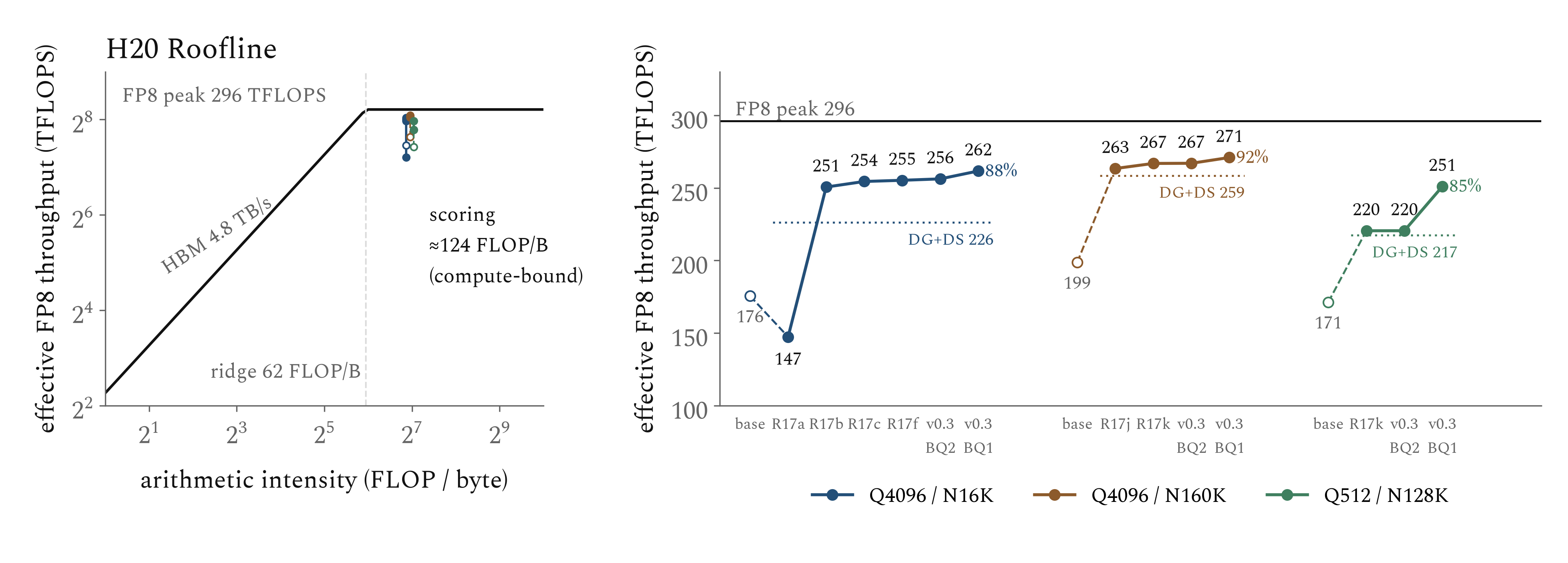
Figure 1: Roofline and version trajectory on H20-3e. Left: every version has the same arithmetic intensity (about 124 FLOP/B), in the compute-bound region right of the ridge at 62. Right: effective throughput on the same inputs with the same protocol (eager); hollow points are the unfused DeepGEMM + torch.topk, dotted lines DeepGEMM + DeepSelect.
| Shape | Unfused (torch.topk) | Fused versions | Public v0.3.0 | DeepGEMM + DeepSelect |
|---|---|---|---|---|
| Q4096 / N16K (1 input) | 176 (59%) | R17a 147 → R17b 251 → R17c 254 → R17f 255 | 262 (88%) | 226 |
| Q4096 / N160K (20 inputs) | 199 (67%) | R17j 263 → R17k 267 | 271 (92%) | 259 |
| Q512 / N128K (1 input) | 171 (58%) | R17k 220 | 251 (85%) | 217 |
Table 8a: Effective FP8 throughput (TFLOPS, eager); percentages are of the 296 TFLOPS spec peak. CUDA Graph differs from eager by only 1–2 TFLOPS.
- Start: the unfused pipelines reach only 58%–67% of peak. They are compute-bound too; they are slow because scoring and top-k run serially.
- The R17a dip: removing the intermediate matrix but making Math wait for TopK drops 176 to 147. Saving traffic is not the same as being fast.
- The R17b jump: double-buffered overlap lifts it to 251, the largest step in the figure. The value of fusion is overlap.
- Small steps afterwards: the exception path (263 → 267 at 160K) and the scheduling tail (220 → 251 at Q512).
- Ceiling: 160K reaches about 92% of peak. Against DeepGEMM + DeepSelect, the three shapes are about 1.16×, 1.05× and 1.15×.
5.2 Math-only control: how much selection time is still exposed
On a copy of the public main kernel we kept the TMA loads, WGMMA and barriers and removed score reduction, candidate generation and top-k. The WGMMA accumulators are folded into a checksum that is written out, so the compiler cannot delete the matrix computation. NCU on Q4096 / H128K confirms that both versions execute identical dynamic QGMMA (68,190,208) and TMA load (4,265,984) instruction counts, while total SASS instructions drop by 85.4%.
| Q | History | Main-kernel speedup after removing all selection |
|---|---|---|
| 8192 | 128K | 0.20% |
| 4096 | 128K | 0.31% |
| 4096 | 24K | 1.64% |
| 512 | 128K | 2.00% |
| 512 | 8K | 21.75% |
Table 9: Math-only control. Synthetic input, timed alternately with the unmodified version in the same rounds.
85% fewer instructions, only 0.31% less time: with long histories, the selection work is almost entirely off the critical path. Note that this number is “the selection time still exposed on the current matrix path”, not the cost of selection itself, and not an upper bound for every possible optimization. With short histories the matrix work cannot cover selection, and removing selection still saves 21.75%.
5.3 Main-kernel compute utilization
| Q | N | Effective TFLOPS | Of peak | SMs used | TopK busy fraction |
|---|---|---|---|---|---|
| 4096 | 8K | 264 | 89.1% | 78 | 0.85 |
| 4096 | 16K | 273 | 92.2% | 78 | 0.43 |
| 4096 | 32K | 277 | 93.5% | 78 | 0.19 |
| 4096 | 64K | 279 | 94.1% | 78 | 0.09 |
| 4096 | 128K | 279 | 94.4% | 78 | 0.05 |
| 4096 | 160K | 282 | 95.2% | 78 | 0.04 |
| 512 | 128K | 261 | 88.1% | 78 | 0.05 |
| 64 | 128K | 220 | 74.4% | 64 | 0.04 |
| 8 | 128K | 28 | 9.4% | 8 | 0.04 |
Table 10: Public main kernel (sampling and repair excluded), real replay rows, fixed threshold, 20 timing groups. The six Q4096 rows come from one measurement (2026-10-13); the last three from an earlier one (2026-10-05). Shapes measured in both runs, Q4096 / N8K at 89.1% vs 88.7% and N32K at 93.5% in both, indicate run-to-run repeatability. TopK busy fraction = time TopK warps spend processing candidates ÷ (processing time + time waiting for candidates to become ready), from a separate instrumented launch; use it for trends only.
At Q4096 all 78 SMs have work, and the main kernel rises from 89.1% at 8K to 95.2% at 160K. The last column explains why: at 8K the TopK warps spend 85% of their time processing candidates and barely keep up with scoring; from 64K on it is under 10%, and they mostly wait for Math to produce the next batch. This agrees with Section 5.2: the longer the history, the more matrix work each row has to cover selection.
When Q is smaller than the SM count, per-query parallelism runs out: Q64 uses only 64 SMs and Q8 only 8, and an idle TopK cannot help because parallelism is the bottleneck. In the 2026-10-05 measurement, Q128 / Q256 (N128K) used all SMs yet reached only 75.1% / 76.8%: 128 and 256 rows do not divide evenly over 78 SMs, so the busiest SM processes one extra row, the scheduling tail of Section 4.6.
Summary: in the main regime of long context and large Q the pipeline is full and this approach is close to its ceiling; further large gains require doing less matrix work. The remaining limits are “short histories cannot hide selection” and “small Q lacks parallelism”.
6 Evaluation
6.1 Setup
- Version under test: public release v0.3.0, commit
05b44daa14991d241de26162aa1bcb773cb6dafb, built from a clean checkout and not modified during measurement. - Baselines: DeepGEMM (
7c95b14a) scoring + DeepSelect (0f03b687) top-k, i.e. the unfused pipeline; native vLLM additionally in the end-to-end test. - Environment: NVIDIA H20-3e, PyTorch 2.10.0+cu130. B=1, 64 heads, dim 128, K=2048.
- Inputs: 240 real activation replays from DeepSeek-V3.2 layers 0/15/30/45/60 at six lengths (8K–160K): 120 at Q4096 and 60 each at Q64 and Q512 (suffix slices of the original activations). 46 synthetic inputs are used only for shape and correctness checks.
- Timing protocol: complete operator, i.e. sampling gather, sampling GEMM, threshold, fused main kernel and exact repair. 7 groups of CUDA events with the same inputs in rotated paired order; warm cache, no L2 flush. JIT, preparation and Graph capture are not timed. Eager and CUDA Graph are measured separately and Graph is reported. GPU clocks were not locked.
6.2 Operator performance
| N | Ours (ms) | DeepGEMM + DeepSelect (ms) | Speedup |
|---|---|---|---|
| 8K | 1.795 | 1.872 | 1.04× |
| 16K | 3.685 | 4.258 | 1.16× |
| 32K | 7.722 | 8.694 | 1.13× |
| 64K | 15.761 | 17.131 | 1.09× |
| 128K | 31.912 | 33.738 | 1.06× |
| 160K | 39.836 | 41.870 | 1.05× |
Table 11: Q4096 complete-operator time (CUDA Graph). Each N is the arithmetic mean of per-input medians over 20 inputs; speedup = baseline ÷ ours.
| Q | Inputs | vs DeepGEMM + DeepSelect (geometric mean) |
|---|---|---|
| 64 | 60 | 1.561× |
| 512 | 60 | 1.125× |
| 4096 | 120 | 1.086× |
Table 12: Geometric mean of per-case speedups by Q. 1.086× should not be read as “8.6% less time”.
vLLM’s usual chunked-prefill budget is 8192 tokens, so Q8192 is a shape that really occurs. The real activations were captured with only 4096 queries each, so Q8192 exists only as synthetic input:
| N | Ours (ms) | DeepGEMM + DeepSelect (ms) | Speedup |
|---|---|---|---|
| 16K | 6.216 | 7.356 | 1.18× |
| 32K | 14.163 | 16.274 | 1.15× |
| 64K | 30.057 | 32.800 | 1.09× |
| 128K | 62.256 | 65.133 | 1.05× |
| 160K | 77.704 | 81.474 | 1.05× |
Table 12b: Synthetic Q8192 (CUDA Graph), mean of the medians of two random seeds. Q8192 / N8K is not measured because some rows have fewer than K valid keys. Synthetic input does not replace real activations; it only confirms that the trend matches Q4096.
- All 120 Q4096 inputs are faster than the unfused pipeline. The speedup shrinks as N grows, for the reason in Section 5.2: at long N both pipelines do the same matrix work, and only the intermediate matrix and the serial stage remain to separate them.
- The Q4096 conclusion is the same in eager mode (1.081×).
- Under Graph, the median coefficient of variation across repeat groups is 0.06%–0.12%.
6.3 Correctness
- All 286 inputs (240 real and 46 synthetic) pass per-row bounds and uniqueness checks.
- An independent oracle (DeepGEMM scoring plus
torch.topk) checks the first, middle and last row of each input as well as every row whose index set differs between implementations, comparing the sorted K scores element by element; 852 case-rows were audited on real inputs. - On real Q4096, 10 rows failed the fast path (0.00203% of 491,520), all fixed by repair; there are no unresolved failures.
These checks are not an independent oracle on every row, and they do not prove token-identical model generations.
6.4 End to end: TTFT
Setup:
- One loaded DeepSeek-V3.2 in one vLLM process (vLLM 0.28.0); only the prefill Indexer is replaced and decode stays native.
- 6×H20-3e, TP2 / PP3, eager, concurrency 1; FP8 weights,
fp8_ds_mlaKV cache, prefix cache off, chunked-prefill budget 8192. - Two real inputs per length, 8 generated tokens per request. Implementations rotate in Williams order, 8 rounds per case.
- TTFT runs from request submission to the first non-empty token and includes scheduling, communication, adapter checks, sampling and repair.
| Input length | Native vLLM | DeepGEMM + DeepSelect | Ours | vs native |
|---|---|---|---|---|
| 8K | 2.751 | 2.762 | 2.761 | fused path not invoked |
| 16K | 4.029 | 4.086 | 4.022 | −0.19% |
| 32K | 6.653 | 6.773 | 6.628 | −0.36% |
| 64K | 12.963 | 13.220 | 12.883 | −0.62% |
| 128K | 29.886 | 30.433 | 29.396 | −1.64% |
Table 13: TTFT (seconds), mean of the two inputs’ medians. Per-case paired bootstrap 95% intervals are narrow (e.g. 1.0162× to 1.0169× at 128K), but they reflect only within-session repeatability; two inputs do not represent the corpus.
- Native vLLM is a strong baseline: it already uses DeepGEMM scoring plus a dedicated prefill top-k, not
torch.topk. - 8K: early causal rows have fewer than K valid keys, so the adapter falls back to native for everything and there is no gain. Both implementations that go through the adapter are about 0.4% slower at 8K, which points to the adapter’s fixed overhead.
- 160K is not in the table: the original 160K inputs ran past the position range in the following decode phase, which native also reproduced, so they are excluded from the formal comparison.
- The 8 generated tokens are not always identical across implementations: exact top-k allows any choice among ties, which does not imply equal task quality.
6.5 Magnitude check
The end-to-end gain should be roughly the Indexer’s share times the operator’s saving relative to native:
| Input length | Native Indexer share | Saving vs native | Estimate | Measured TTFT reduction |
|---|---|---|---|---|
| 16K | 9.62% | 5.99% | ≈ 0.6% | 0.19% |
| 32K | 16.78% | 4.33% | ≈ 0.7% | 0.36% |
| 64K | 28.37% | 3.42% | ≈ 1.0% | 0.62% |
| 128K | 44.11% | 4.43% | ≈ 2.0% | 1.64% |
Table 14: The saving is the reduction in Indexer GPU work of the fused version relative to native over the many Q/N shapes actually invoked, including sampling, repair and adapter checks.
The two agree in magnitude and both grow with length. The measurement falls below the estimate for several reasons:
- the share is computed from summed kernel time over six GPUs, not the critical path;
- the first 8192-token chunk falls back to native, 122 such calls per request;
- TTFT also includes CPU scheduling, communication and adapter overhead.
The end-to-end gain is therefore capped by the Indexer’s share.
7 Lessons: where expectation and measurement disagreed
| Attempt | Expected | Measured | Lesson |
|---|---|---|---|
| Heap maintenance | , catch up with FlashInfer | Half the instructions, but 128K still 4.220 ms, slower than FlashInfer | Lower complexity does not remove maintenance |
| Index-only storage | Less SMEM, so faster | All eight test points 2.60%–13.54% slower | Residency follows thresholds, not usage |
| First on-chip fusion | No round trip, so faster | 6.616 ms, slower than unfused (147 vs 176 TFLOPS) | Fusion must design who waits for whom |
| Scanning actual counts | TopK 26% faster, so overall clearly faster | Complete operator only 1.09% faster | TopK was already hidden by the pipeline |
| One query per batch | Narrower MMAs are more efficient | Per-query cycles unchanged; the busiest SM does one row less | Metrics need intervention experiments |
| Hand-cut instructions | Fewer instructions, so faster | Static SHFL 20 → 15, FADD 30 → 25, no reliable end-to-end change | Instruction count is not time |
Table 15: Six judgments overturned by data. Each row maps to a section above; their measurement scopes differ, so numbers are not compared across rows.
One lesson runs through all of them: find the path that determines total time before acting on it. When a metric improves, first ask whether it is on that path, then whether the numerator or the denominator changed.
8 Limitations
- Gains depend on shape: the speedup is smallest at long N (about 1.05× at 160K) because the scoring matrix work dominates. At small Q and short histories the SMs are underused and selection is not hidden.
- Fusion is incomplete: only the main kernel is fused. Each call still goes through five stages: sampling gather, sampling GEMM, threshold, main kernel and repair. Even with zero failures, masked repair launches several kernels (5 at 8K, 26 at 128K), about 0.357 ms or roughly 0.9% at 160K. These fixed costs are more visible at small Q.
- Performance depends on the data distribution: exactness is guaranteed by the certificate and repair regardless of distribution, but performance depends on how well the threshold is estimated. With a different sampling seed, underflow still appears in layer 60 of the 160K development set.
- Scope of support and validation:
- only Hopper (H20) FP8 with B=1 / 64 heads / dim 128 / K=2048 and N from 8K to 160K;
- the real inputs come from one capture: 24 prompts, 1032 source documents, five layers;
- real Q8192 was not measured (synthetic Q8192 shows a Q2 ÷ Q1 of only 1.004×).
- Only TTFT is validated: each request generates 8 tokens, which says nothing about decode throughput, concurrent TPS or tail latency.
9 Related work
- DeepGEMM provides the FP8 MQA logits kernel and the TMA / WGMMA pipeline and SMEM layout this project builds on.
- DeepSelect and FlashInfer top-k are standalone top-k kernels whose input is a full score matrix already in device memory. They are the baselines for this project’s standalone top-k stage; the “write then read back” boundary they sit on is exactly what the fusion stage removes.
- vLLM’s DSA implementation, DeepGEMM scoring plus a dedicated prefill top-k, is the native baseline in the end-to-end experiment.
- FlashAttention fuses the production and consumption of attention scores into one kernel to avoid materializing an matrix. This project faces a similar producer–consumer fusion, but the consumer is an exact top-k, which cannot reuse softmax’s online recurrence; hence bounded candidates plus exact recovery.
- NSA and HISA: NSA selects contiguous blocks so that sparse access is regular by construction. HISA reduces Indexer compute with hierarchical block-level filtering and reports a 1.70× TTFT speedup on 8×H200, but it changes the selection semantics. This project keeps exact semantics and optimizes the implementation.
10 Conclusion
Removing the intermediate matrix is only the starting point. On H20, Indexer scoring is compute-bound, so the value of fusion lies mainly in overlapping exact selection with scoring rather than in saving bandwidth. To get there, we first changed top-k from online maintenance to sampled filtering plus exact selection over a small set, then put it into the scoring pipeline with warp specialization and double buffering, and removed candidate-write contention, empty-slot scans, overflow recomputation and scheduling tails in turn. The complete operator reaches about 92% of FP8 peak, selection is almost fully hidden at long histories, the operator is consistently faster than the unfused pipeline on real activations, and inside vLLM it turns into a TTFT gain consistent with the estimate.
The remaining room on the prefill side has to come from doing less matrix work; small Q and decode need parallelism split along the KV dimension.
Appendix A: Reproduction
| Item | Value |
|---|---|
| Public release | v0.3.0, 05b44daa14991d241de26162aa1bcb773cb6dafb |
| DeepGEMM | 7c95b14aa4a66edd7b682e5acdde62351ca81197 |
| DeepSelect | 0f03b68748b304863fdf0181a11458d04ae533a9 |
| Operator environment | NVIDIA H20-3e, PyTorch 2.10.0+cu130 |
| End-to-end environment | vLLM 0.28.0, PyTorch 2.13.0+cu132, 6×H20-3e, TP2 / PP3 |
Appendix B: Timing scopes
| Section | Scope |
|---|---|
| 3 (standalone top-k) | Sum of CUPTI kernel time over the top-k stage, including sampling, filtering, selection, output and repair; real Layer-0 score replay |
| 4 (fused design) | Warm median of complete-operator CUDA events, 24 alternating groups; cycles from a separate instrumented build |
| 5.1 (version trajectory) | Complete operator, eager, CUDA events; same inputs, rotated |
| 5.2, 5.3 (main kernel) | Main kernel only, sampling and repair excluded |
| 6.2 (operator) | Complete operator, CUDA Graph, 7 paired groups |
| 6.4 (end to end) | Whole-model TTFT, eager, concurrency 1, 8 Williams-ordered rounds |
Numbers are compared only within the same scope.